Sage Journals: Discover world-class research

Abstract

In this paper, a novel modeling and parameter learning method for the Hammerstein–Wiener model with disturbance is proposed, and the Hammerstein–Wiener model is implemented to approximate complex nonlinear industrial processes. The proposed Hammerstein–Wiener model has two static nonlinear blocks represented by two independent neuro-fuzzy models that surround a dynamic linear block described by the finite impulse response model. The parameter learning method of the Hammerstein–Wiener model with disturbance can be summarized in the following three steps: First, the designed input signals are implemented to completely separate the parameter learning problem of output nonlinear block, linear block, and input nonlinear block. Meanwhile, the static output nonlinear block parameters can be learned based on input and output data of two sets of separable signals with different sizes. Second is to determine the dynamic linear block parameter using correlation analysis algorithm using one set of separable signal; thus, the process disturbance can be compensated by the calculation of correlation function. The final one is to achieve unbiased estimation of the static input nonlinear block parameters using least squares method according to the input–output data of random signal. Furthermore, with the parameter learning method, the proposed model can achieve less computation complexity and good robustness. The simulation results of two cases are provided to demonstrate the advantage of the proposed modeling and parameter learning method.

Keywords

Hammerstein–Wiener model process disturbance designed input signals parameter learning

Introduction

Almost all practical industrial processes have nonlinear characteristics to some extent.^1,2 For decades, many methodologies have been carried out in the field of nonlinear dynamic system modeling and identification, for example, Volterra series,³ block-oriented nonlinear models,^4–12 neural networks,^13,14 support vector machines,^15,16 and Markov jump systems.¹⁷ Among these methodologies, block-oriented nonlinear models have received widespread attention due to their simple structure and excellent modeling ability.¹⁸

The Hammerstein and Wiener models represent the most familiar models of the nonlinear block-oriented models. The extension of the Hammerstein and Wiener models is the Hammerstein–Wiener model, which constituted by one dynamic linear block surrounded by two static nonlinear blocks has a great flexibility for describing practical nonlinear systems, such as electric arc furnace system,¹⁹ pH neutralization process,^20,21 continuous stirred tank reactor (CSTR),²² and fermentation bioreactor system.²³ There is an extensive body of research with regard to various learning algorithms of the Hammerstein–Wiener model, mainly including over-parameterization method,²⁴ subspace method,²³ blind method,²⁵ iterative method,^26,27 multi-signal based method,²⁸ and maximum likelihood method.²⁹

In the work by Bai,²⁴ a two-stage parameter learning method based on least squares method and singular value decomposition technology was proposed for the Hammerstein–Wiener model: the first stage carries out parameter learning of an augmented model, and the second stage separates the unknown parameters of the linear and nonlinear parts using singular value decomposition. Vörös²⁷ employed least squares–based iterative approach to learn the parameters of the three-block cascade model with output backlash. A new recursive algorithm is derived for the learning of the Hammerstein–Wiener model with dead-zone nonlinearity as input block and polynomial function nonlinearity as output block as in the work by Yu et al.³⁰ Zhang et al.³¹ developed recursive least squares (RLS) algorithm to learn the parameters of the Hammerstein–Wiener model using the key-term separation principle, and the adaptive controller was designed. However, the common representation of the methods mentioned is that the Hammerstein–Wiener model’s learning process contains unknown parameter product of static nonlinear blocks and dynamic linear block, which increases the learning complexity and computational burden. Furthermore, the process disturbance of the Hammerstein–Wiener model is not considered explicitly, which is not consistent with the characteristics of the practical industrial processes. Different from the output disturbance of the model, process disturbance is placed before the static output nonlinear block, which indicates that the output disturbance is large when the process gain is large; on the contrary, the output disturbance is small when the gain is small.³² From the perspective of process operation, it is more realistic to consider process disturbance.

The least squares methods are the dominant algorithms for system identification and parameter learning of nonlinear dynamic models owing to their simplicity in concept and convenience in implementation. Recently, the RLS methods have been applied for the parameter learning of the Hammerstein–Wiener model. It is acknowledged that RLS methods are unable to generate consistent estimation of the model parameters when the model involves process noise or measurement noise. For this reason, various modified RLS learning schemes have been developed.^33–35 Based on the hierarchical identification principle and the auxiliary model identification idea, Wang and Ding³³ presented hierarchical least squares method to learn the Hammerstein–Wiener output error model parameter. Bias compensation principle is combined with the singular value decomposition method for learning the Hammerstein–Wiener model, and an improved online two-stage identification algorithm is introduced in the work by Li et al.³⁴ By extending the simplified and refined instrumental variable method, Allafi et al.³⁵ studied the instrumental variable least squares parameter estimation algorithm for the fractional-order Hammerstein–Wiener model. It should be noted that the abovementioned results assumed that unknown static nonlinearities are of polynomial forms. Consequently, if the nonlinear blocks are not polynomial forms or not continuous functions, the approaches do not converge.³⁶

To circumvent the aforementioned problem, fuzzy model and neural network model have been developed for representing nonlinear blocks of the Hammerstein–Wiener model because of their strong approximation ability for nonlinear functions. Therefore, it is worth emphasizing that the parameter learning of fuzzy system– or neural network–based Hammerstein–Wiener model has essential differences from the parameter learning of single fuzzy model or single neural network model, the difference being that the model structure constraint was imposed by the nonlinear Hammerstein–Wiener model. The parameter learning problem of the Hammerstein–Wiener model needs to take into account nonlinear transformations and linear dynamics altogether, while the parameter learning of the traditional neuro-fuzzy systems only focuses on one global nonlinear transformation. Chen and Wang³⁷ reported a Hammerstein–Wiener recurrent neural network, in which systematic identification algorithm is used to identify unknown dynamic nonlinear systems. Combining the back-propagation technique with stochastic gradient algorithm, Abouda et al.³⁸ researched the parameter learning method of estimating jointly unknown parameters and the intermediate variable of fuzzy Hammerstein–Wiener model. However, neural network models have strong self-learning and self-adaptive ability, but lacks transparency and cannot well express the reasoning capability of human brain, while the fuzzy system has no self-adaptive ability, and it has some boundedness in practical applications. The neuro-fuzzy model integrates the learning mechanism of neural networks with the ability of fuzzy inference technology, which can better describe the nonlinear dynamic systems than neural networks or fuzzy systems. As a result, a significant idea is to use the neuro-fuzzy model as static nonlinear blocks of the Hammerstein–Wiener model.

To deal with the issues described above, a novel modeling and parameter learning method for the Hammerstein–Wiener model with disturbance is considered, whose two static nonlinearities are represented using two independent four-layer neuro-fuzzy models, while a dynamic linear block is described using the finite impulse response model. The designed input signals are utilized to achieve the decoupling of parameter learning of output nonlinear block, linear block, and input nonlinear block. First, the output static nonlinear block parameters can be estimated using two sets of separable signals with different sizes. Moreover, correlation analysis approach is developed for determining the unknown parameters of linear block. Finally, parameter unbiased estimation of the static input nonlinear block is achieved using least squares method based on input and output random signals. The main contributions of this paper are as follows:

In our previous work,³⁹ the input signals that consist of binary signal and random multistep signal are used to identify the Hammerstein–Wiener model. In contrast, in this work, the first part of the special input signal is extended to include more general independent separable signals, such as binary signal, sine signal, and Gaussian signal.

Unlike the synchronous parameter learning methods,^23,24 the designed input signals are implemented to completely separate the parameter learning problem of output nonlinear block, linear block, and input nonlinear block, which significantly simplifies the parameter learning process of the Hammerstein–Wiener model.

The correlation analysis algorithm is employed to learn the unknown parameters of the dynamic linear block; thus, the process disturbance can be compensated by the calculation of correlation function.

The modeling and parameter learning problem of the Hammerstein–Wiener model is briefly presented in section “The neuro-fuzzy Hammerstein–Wiener model.” The three-stage parameter learning algorithms of the neuro-fuzzy Hammerstein–Wiener model with disturbance are discussed carefully in section “Parameter learning of the neuro-fuzzy Hammerstein–Wiener model.” Section “Simulation results and analysis” gives the simulation results of complex nonlinear industrial processes. Finally, we draw some conclusions in section “Conclusion.”

The configuration of neuro-fuzzy Hammerstein-Wiener model

The Hammerstein–Wiener model

As depicted in Figure 1, we consider the following Hammerstein–Wiener model with disturbance³³ that consists of one dynamic linear block, $H (\cdot)$ , surrounded by input static nonlinear block, $f (\cdot)$ , and output static nonlinear block, $g (\cdot)$ .

Figure 1.

Structure of the Hammerstein–Wiener model.

The Hammerstein–Wiener model, defined in Figure 1, is expressed by the relationships of three blocks

$v (k) = f (u (k))$ (1)

$x (k) = H (z) v (k)$ (2)

$z (k) = x (k) + e (k)$ (3)

$y (k) = g (z (k))$ (4)

where $f (\cdot)$ is the static input nonlinear block; $H (z)$ is the dynamic linear block; $g (\cdot)$ is the static output nonlinear block; $e (k)$ is a white noise with zero mean and unknown variance $σ^{2}$ ; $v (k)$ , $x (k)$ , and $z (k)$ are the intermediate variables of the model; and $u (k)$ and $y (k)$ denote the input and output, respectively.

In the dynamic block, the current output depends on its past values. The dynamic linear block can be described as a finite impulse response, space state model, transfer function, and so on. Here, a finite impulse response model is considered, that is, $B (z) = b_{1} z^{- 1} + b_{2} z^{- 2} + \dots + b_{n_{b}} z^{- n_{b}}$ , where $z^{- 1}$ represents the unit delay operator and $n_{b}$ represents the model order.

In the parameter learning method of the Hammerstein–Wiener model, a crucial challenge is to discover an effective representation of static nonlinear blocks. A good modeling should not only correctly represent the static nonlinear block but also simplify the parameter learning procedure. By analyzing the superiorities of fuzzy systems and neural network models in section “Introduction,” the proposed neuro-fuzzy models are applied to the Hammerstein–Wiener model with disturbance in the next study.

The neuro-fuzzy Hammerstein–Wiener model

Four-layer neuro-fuzzy models are designed to formulate static input nonlinear block and static output nonlinear block, as shown in Figure 2.

Figure 2.

The neuro-fuzzy model.

Furthermore, the intermediate variables $v (k)$ and $z (k)$ are defined as

$\hat{v} (k) = \hat{f} (u (k)) = \sum_{l = 1}^{L^{input}} ϕ_{l}^{input} (u (k)) w_{l}^{input}$ (5)

$\hat{z} (k) = {\hat{g}}^{- 1} (y (k)) = \sum_{l = 1}^{L^{o u t p u t}} ϕ_{l}^{o u t p u t} (y (k)) w_{l}^{o u t p u t}$ (6)

where $ϕ_{l}^{input} (u (k)) = (μ_{l} (u (k))) / (\sum_{l = 1}^{L^{input}} μ_{l} (u (k)))$ and $ϕ_{l}^{o u t p u t} (y (k)) = (μ_{l} (y (k))) / (\sum_{l = 1}^{L^{o u t p u t}} μ_{l} (y (k)))$ , in which $μ_{l} = \exp (- (u (k) - c_{l})^{2}) / σ_{l}^{2}$ , $c_{l}$ is the center, $σ_{l}$ is the width, $w_{l}^{input} (l = 1, 2, . . ., L^{input})$ is the weight of the input nonlinear block, $L^{input}$ is the total fuzzy rule, $w_{l}^{o u t p u t} (l = 1, 2, . . ., L^{o u t p u t})$ is the weight of the output nonlinear block, and $L^{o u t p u t}$ is the fuzzy rule of the neuro-fuzzy model.

According to the given structure of the Hammerstein–Wiener model, the neuro-fuzzy Hammerstein–Wiener system consists of two static nonlinear blocks described by two independent neuro-fuzzy models and a dynamic linear block described by finite impulse response model. The elaborate structure is shown in Figure 3.

Figure 3.

Configuration of neuro-fuzzy Hammerstein–Wiener system.

For the available observed data set and given order $n_{b}$ , a common method for parameter learning is to find the best fit of the Hammerstein–Wiener model by minimizing the loss function

$\begin{array}{l} E (\hat{f} (u (k)), {\hat{b}}_{1}, ..., {\hat{b}}_{n_{b}}, \hat{g} (\hat{z} (k))) = \frac{1}{2 N} {\sum_{k = 1}^{N} [y (k) - \hat{y} (k)]}^{2} \leq ε \\ s . t . \\ \hat{v} (k) = \hat{f} (u (k)) \\ \hat{z} (k) = \hat{B} (z) \hat{v} (k) + e (k) \\ \hat{y} (k) = \hat{g} (\hat{z} (k)) \end{array}$ (7)

where $\hat{v} (k)$ and $\hat{z} (k)$ are the intermediate variable estimation, $\hat{f} (\cdot)$ is the input nonlinear block estimation, $\hat{g} (\cdot)$ is the output nonlinear block estimation, $ε$ is the given tolerance, and $N$ is the total observed data.

Parameter learning of the neuro-fuzzy Hammerstein–Wiener model

In this section, a parameter learning process of neuro-fuzzy Hammerstein–Wiener model with disturbance using designed input signals is concretely discussed. The objective of the proposed learning method is to acquire the parameter estimation of three blocks.

The designed input signals are made up of separable signals and random signals, which are implemented to activate the Hammerstein–Wiener model, bringing out completely the parameter learning of three blocks (i.e. output nonlinear block, linear block, and input nonlinear block). In the parameter learning of the Hammerstein model, from the perspective of static nonlinear block, our previous research work⁴ has demonstrated the relationship of input–output signals under separable signals. Taking advantage of the idea of this work, further research of the Hammerstein–Wiener model is discussed.

Theorem 1

With the static input nonlinear block of the Hammerstein–Wiener model, if the model input $u (k)$ is the separable signal, then there is a constant $b_{0}$ which makes the following equation hold

$R_{vu} (τ) = b_{0} R_{u} (τ), \forall τ \in Z$ (8)

where $R_{vu} (τ) = E (v (k) u (k - τ))$ denotes the function constituted by input signal and corresponding output signal, $R_{u} (τ) = E (u (k) u (k - τ))$ denotes the function composed of input signal, and $b_{0} = E (v (k) u (k)) /$ $E (u (k) u (k))$ denotes constant.

The certification process of Theorem 1 can be done by referring to the method by Li and Jia⁴ and hence it is omitted here.

Theorem 1 shows that $R_{vu} (τ)$ constituted by model input signal and intermediate signal can be replaced by $R_{u} (τ)$ composed of model input signal. Two advantages can be obtained from Theorem 1: first, the parameter learning of static input nonlinear block and the Wiener model (i.e. combination of dynamic linear block and static output nonlinear block) are implemented. Second, the problem that the information of the intermediate variable $v (k)$ is not measurable can be effectively solved.

Based on the above analysis, the parameter learning process of the Hammerstein–Wiener model with process disturbance is specifically analyzed.

Learning the static output nonlinear block parameters

In this subsection, the result of Theorem 1 is employed in the Hammerstein–Wiener model. Two sets of separable input and output signals with different sizes are adopted to learn the parameters of the static nonlinear block. In the parameter learning process, we need to determine the center, $c_{l}^{o u t p u t}$ , the width, $σ_{l}^{o u t p u t}$ , and the weight, $w_{l}^{o u t p u t}$ , of the static output nonlinear block represented by neuro-fuzzy model. The center, $c_{l}^{o u t p u t}$ , and the width, $σ_{l}^{o u t p u t}$ , can be computed using the cluster method previously proposed.⁴⁰ To this end, the key challenge is how to estimate the weight, $w_{l}^{o u t p u t}$ .

The output signals $y_{1} (k)$ and $y_{2} (k)$ , corresponding to two sets of input signals with different sizes, are used. The static output nonlinear block can be expressed as

$z_{1} (k) = {\hat{g}}^{- 1} (y_{1} (k)) = \sum_{l = 1}^{L_{1}^{o u t p u t}} ϕ_{l}^{o u t p u t} (y_{1} (k)) w_{l}^{o u t p u t}$ (9)

$z_{2} (k) = {\hat{g}}^{- 1} (y_{2} (k)) = \sum_{l = 1}^{L_{2}^{o u t p u t}} ϕ_{l}^{o u t p u t} (y_{2} (k)) w_{l}^{o u t p u t}$ (10)

According to equations (2) and (3), equations (9) and (10) can be rewritten into a linear regression form as

$z_{1} (k) = \sum_{j = 1}^{n_{b}} b_{j} v_{1} (k - j) + e (k)$ (11)

$z_{2} (k) = \sum_{j = 1}^{n_{b}} b_{j} v_{2} (k - j) + e (k)$ (12)

Multiplying both sides of equations (11) and (12) by $u_{1} (k - τ)$ and $u_{2} (k - τ)$ , respectively, and calculating the mathematical expectations, we get

$R_{z_{1} u_{1}} (τ) = \sum_{j = 1}^{n_{b}} b_{j} R_{v_{1} u_{1}} (τ - j) + R_{e u_{1}} (τ)$ (13)

$R_{z_{2} u_{2}} (τ) = \sum_{j = 1}^{n_{b}} b_{j} R_{v_{2} u_{2}} (τ - j) + R_{e u_{2}} (τ)$ (14)

$e (k)$ is independent of system input signal, $u (k)$ and $u_{2} (k)$ ; therefore, $R_{e u_{1}} (τ) = 0$ and $R_{e u_{2}} (τ)$ . Furthermore

$R_{z_{1} u_{1}} (τ) = \sum_{j = 1}^{n_{b}} b_{j} R_{v_{1} u_{1}} (τ - j)$ (15)

$R_{z_{2} u_{2}} (τ) = \sum_{j = 1}^{n_{b}} b_{j} R_{v_{2} u_{2}} (τ - j)$ (16)

Using Theorem 1, we obtain

$R_{z_{1} u_{1}} (τ) = \sum_{j = 1}^{n_{b}} b_{01} b_{j} R_{u_{1}} (τ - j)$ (17)

$R_{z_{2} u_{2}} (τ) = \sum_{j = 1}^{n_{b}} b_{02} b_{j} R_{u_{2}} (τ - j) = λ^{2} \sum_{j = 1}^{n_{b}} b_{02} b_{j} R_{u_{1}} (τ - j)$ (18)

where $b_{01} = (E (v_{1} (k) u_{1} (k))) / (E (u_{1} (k) u_{1} (k)))$ and $b_{02} = (E (v_{2} (k) u_{2} (k))) / (E (u_{2} (k) u_{2} (k)))$ .

Combining equation (17) with equation (18) yields

$R_{z_{2} u_{2}} (τ) = β R_{z_{1} u_{1}} (τ)$ (19)

where $λ = u_{2} / u_{1}$ and $β = λ^{2} b_{01} / b_{02}$ .

Furthermore, equation (29) can be defined as

$E (z_{2} (k) u_{2} (k - τ)) = β E (z_{1} (k) u_{1} (k - τ))$ (20)

Substituting equations (9) and (10) into equation (20), we obtain

$\sum_{l = 1}^{L^{o u t p u t}} w_{l}^{o u t p u t} E (ϕ_{l}^{o u t p u t} (y_{2} (k)) u_{2} (k - τ)) = β \sum_{l = 1}^{L^{o u t p u t}} w_{l}^{o u t p u t} E (ϕ_{l}^{o u t p u t} (y_{1} (k)) u_{1} (k - τ))$ (21)

Let $ϕ_{l, i}^{o u t p u t} (k) = ϕ_{l}^{o u t p u t} y_{i} (k)$ $(l = 1, . . ., L^{o u t p u t}; i = 1, 2)$ , then

$\sum_{l = 1}^{L^{o u t p u t}} w_{l}^{o u t p u t} R_{ϕ_{l, 2}^{o u t p u t} u_{2}} (τ) = β \sum_{l = 1}^{L^{o u t p u t}} w_{l}^{o u t p u t} R_{ϕ_{l, 1}^{o u t p u t} u_{1}} (τ)$ (22)

Dividing both sides of equation (22) by $w_{1}^{o u t p u t}$ , we get

$\begin{matrix} R_{ϕ_{1, 2}^{o u t p u t} u_{2}} (τ) - β R_{ϕ_{1, 1}^{o u t p u t} u_{1}} (τ) \\ = \frac{β \sum_{l = 2}^{L^{o u t p u t}} w_{l}^{o u t p u t} R_{ϕ_{l, 1}^{o u t p u t} u_{1}} (τ) - \sum_{l = 2}^{L^{o u t p u t}} w_{l}^{o u t p u t} R_{ϕ_{l, 2}^{o u t p u t} u_{2}} (τ)}{w_{1}^{o u t p u t}} \end{matrix}$ (23)

Let ${\bar{w}}_{l}^{o u t p u t} = w_{l}^{o u t p u t} / w_{1}^{o u t p u t}$ , then

$\begin{matrix} R_{ϕ_{1, 2}^{o u t p u t} u_{2}} (τ) - β R_{ϕ_{1, 1}^{o u t p u t} u_{1}} (τ) \\ = [\sum_{l = 2}^{L^{o u t p u t}} β w_{l}^{o u t p u t} R_{ϕ_{l, 1}^{o u t p u t} u_{1}} (τ) - R_{ϕ_{l, 2}^{o u t p u t} u_{2}} (τ)] {\tilde{w}}_{l}^{o u t p u t} \end{matrix}$ (24)

Assume $τ = 1, 2, . . ., P (P \geq L^{o u t p u t} - 1)$ ; according to equation (19), the following loss function can be described

$E ({\bar{w}}_{l}^{o u t p u t}) = \frac{1}{2 P} \sum_{τ = 1}^{P} {[R_{z_{2} u_{2}} (τ) - β R_{z_{1} u_{1}} (τ)]}^{2}$ (25)

Using least squares method, weight can be obtained by the following formula

${\hat{θ}}_{o u t p u t} = (X^{T} X)^{- 1} X^{T} Y$ (26)

where ${\hat{θ}}_{o u t p u t} = {[{\bar{w}}_{2}^{o u t p u t}, {\bar{w}}_{3}^{o u t p u t}, . . ., {\bar{w}}_{L^{o u t p u t}}^{o u t p u t}]}^{T}$ , $X = [x_{1}, x_{2}, . . ., x_{L^{o u t p u t} - 1}]$ , $x_{l - 1} = [\begin{matrix} β R_{ϕ_{l, 1}^{o u t p u t} u_{1}} (1) - R_{ϕ_{l, 2}^{o u t p u t} u_{2}} (1) \\ β R_{ϕ_{l, 1}^{o u t p u t} u_{1}} (2) - R_{ϕ_{l, 2}^{o u t p u t} u_{2}} (2) \\ \begin{matrix} . \\ . \\ . \end{matrix} \\ β R_{ϕ_{l, 1}^{o u t p u t} u_{1}} (P) - R_{ϕ_{l, 2}^{o u t p u t} u_{2}} (P) \end{matrix}]$ , and $Y = [\begin{matrix} R_{ϕ_{1, 2}^{o u t p u t} u_{2}} (1) - β R_{ϕ_{1, 1}^{o u t p u t} u_{1}} (1) \\ R_{ϕ_{1, 2}^{o u t p u t} u_{2}} (2) - β R_{ϕ_{1, 1}^{o u t p u t} u_{1}} (2) \\ \begin{matrix} . \\ . \\ . \end{matrix} \\ R_{ϕ_{1, 2}^{o u t p u t} u_{2}} (P) - β R_{ϕ_{1, 1}^{o u t p u t} u_{1}} (P) \end{matrix}]$ .

Equations (27) and (28) are used to calculate $R_{ϕ_{l, 1}^{o u t p u t} u_{1}} (τ)$ and $R_{ϕ_{l, 2}^{o u t p u t} u_{2}} (τ)$ , respectively

$R_{ϕ_{l, 1}^{o u t p u t} u_{1}} (τ) = \frac{1}{N} \sum_{k = 1}^{N} \sum_{l = 2}^{L^{o u t p u t}} ϕ_{l, 1}^{o u t p u t} (y_{1} (k)) u_{1} (k - τ)$ (27)

$R_{ϕ_{l, 2}^{o u t p u t} u_{2}} (τ) = \frac{1}{N} \sum_{k = 1}^{N} \sum_{l = 2}^{L^{o u t p u t}} ϕ_{l, 2}^{o u t p u t} (y_{2} (k)) u_{2} (k - τ)$ (28)

Learning the dynamic linear block parameters

The input and output data of separable signals are implemented for learning the unknown parameter of the dynamic linear blocks in this subsection.

According to equation (17), the dynamic linear block can be equivalently rewritten as

$R_{z_{1} u_{1}} (τ) = \sum_{j = 1}^{n_{b}} {\bar{b}}_{j} R_{u_{1}} (τ - j)$ (29)

where ${\bar{b}}_{j} = b_{01} b_{j}$ and $b_{01} = (E (v_{1} (k) u_{1} (k))) / (E (u_{1} (k) u_{1} (k)))$ .

In the last subsection, we have estimated the static nonlinear block parameter, so correlation function, $R_{z_{1} u_{1}} (τ)$ can be computed. Consequently, the correlation analysis algorithm can be utilized to learn linear block unknown parameters.

Assume $τ = 1, 2, . . ., P (P \geq n_{b})$ ; from equation (29), we get

$R = θ_{linear} ψ$ (30)

where $θ_{linear} = [{\bar{b}}_{1}, {\bar{b}}_{2}, . . ., {\bar{b}}_{n_{b}}]$ , $R = [R_{z_{1} u_{1}} (1), R_{z_{1} u_{1}} (2), . . ., R_{z_{1} u_{1}} (P)]$ , and $ψ = [\begin{matrix} R_{u_{1}} (0) & R_{u_{1}} (1) & R_{u_{1}} (2) & . . . & R_{u_{1}} (P - 1) \\ 0 & R_{u_{1}} (0) & R_{u_{1}} (1) & . . . & R_{u_{1}} (P - 2) \\ \begin{matrix} . \\ . \\ . \end{matrix} & \begin{matrix} . \\ . \\ . \end{matrix} & \begin{matrix} . \\ . \\ . \end{matrix} & . . . & \begin{matrix} . \\ . \\ . \end{matrix} \\ 0 & 0 & 0 & . . . & R_{u_{1}} (P - n_{b}) \end{matrix}]$ .

Define a cost function

$E (θ_{linear}) = ‖ R - θ_{linear} ψ ‖^{2}$ (31)

Taking the derivative of equation (31), we obtain

$\begin{matrix} \frac{\partial E (θ_{linear})}{\partial θ_{linear}} = \frac{\partial [{(R - θ_{linear} ψ)}^{T} (R - θ_{linear} ψ)]}{\partial θ_{linear}} \\ = 2 θ_{linear} ψ ψ^{T} - 2 R ψ \end{matrix}$ (32)

Let $\partial E ({θ_{linear}}_{1}) / \partial θ_{linear} = 0$ , we get

$θ_{linear} ψ ψ^{T} = R ψ^{T}$ (33)

Multiplying both sides of equation (33) by the inverse of matrix, $ψ ψ^{T}$ , the parameter estimation is given by

${\hat{θ}}_{linear} = R ψ^{T} (ψ ψ^{T})^{- 1}$ (34)

The following formulas are used to calculate $R_{ϕ_{l, 1}^{o u t p u t} u_{1}} (τ)$ and $R_{ϕ_{l, 2}^{o u t p u t} u_{2}} (τ)$

$R_{z_{1} u_{1}} (τ) = \frac{1}{N} \sum_{k = 1}^{N} \sum_{l = 2}^{L^{o u t p u t}} ϕ_{l, 1}^{o u t p u t} (y_{1} (k)) u_{1} (k - τ)$ (35)

$R_{u} (τ) = \frac{1}{N} \sum_{k = 1}^{N} u (k) u (k - τ)$ (36)

Learning the static input nonlinear block parameters

Based on two sets of separable signals, we have estimated the input nonlinear block parameter and the linear block parameter. Next, we discuss how to learn the static input nonlinear block parameters by means of the available input–output of random signals.

The learning procedure of input nonlinearity characterized by neuro-fuzzy model is to calculate the center, $c_{l}^{input}$ , the width, $σ_{l}^{input}$ , and the weight, $w_{l}^{input}$ . Similar to the previous learning methods of the static output nonlinear block, the center, $c_{l}^{input}$ , and the width, $σ_{l}^{input}$ , can be learned by the cluster method. So an obvious question is whether the weight, $w_{l}^{input}$ , needs to be learned.

From equations (1) and (3), we have

$z (k) = \sum_{j = 1}^{n_{b}} b_{j} v (k - j) + e (k)$ (37)

Using equation (5) yields

$z (k) = \sum_{j = 1}^{n_{b}} \sum_{l = 1}^{L^{input}} b_{j} ϕ_{l}^{input} (u (k - j)) w_{l}^{input} + e (k)$ (38)

For simplicity, equation (38) is rewritten as

$z (k) = φ (k)^{T} θ_{input} + e (k)$ (39)

where $θ_{i n p u t} = {[b_{1} w_{1}^{i n p u t}, ..., b_{1} w_{L}^{i n p u t}, ..., b_{n_{b}} w_{1}^{i n p u t}, ..., b_{n_{b}} w_{L}^{i n p u t}]}^{T}$ and $φ (k) = {[ϕ_{1}^{i n p u t} (u (k - 1)), ..., ϕ_{L}^{i n p u t} (u (k - 1)), ..., ϕ_{L}^{i n p u t} (u (k - n_{b})), ..., ϕ_{L}^{i n p u t} (u (k - n_{b}))]}^{T}$ .

Defining a quadratic cost function according to equation (39)

$J (θ_{input}) = \sum_{k = 1}^{N} {‖ z (k) - φ {(k)}^{T} θ_{input} ‖}^{2}$ (40)

Using least squares estimation method, we get

${\hat{θ}}_{input}^{LS} (k) = {[\sum_{k = 1}^{N} φ (k) φ^{T} (k)]}^{- 1} [\sum_{k = 1}^{N} φ (k) z (k)]$ (41)

According to equations (39) and (41), it is easy to obtain

$\begin{matrix} {\hat{θ}}_{input}^{LS} (k) = {[\sum_{k = 1}^{N} φ (k) φ^{T} (k)]}^{- 1} \\ [\sum_{k = 1}^{N} φ (k) (φ {(k)}^{T} θ_{input} + e (k))] \\ = {[\sum_{k = 1}^{N} φ (k) φ^{T} (k)]}^{- 1} [\sum_{k = 1}^{N} φ (k) φ^{T} (k) θ_{input}] \\ + {[\sum_{k = 1}^{N} φ (k) φ^{T} (k)]}^{- 1} [\sum_{k = 1}^{N} φ (k) e (k)] \\ = θ_{input} + {[\sum_{k = 1}^{N} φ (k) φ^{T} (k)]}^{- 1} [\sum_{k = 1}^{N} φ (k) e (k)] \end{matrix}$ (42)

Note that the noise $e (k)$ is a white noise sequence; therefore

$E [\sum_{k = 1}^{N} φ (k) e (k)] = 0$ (43)

Combing equations (42) and (43), we get

$\begin{matrix} E (θ_{input}^{LS} (k)) = E (θ_{input}) \\ + E [{(\sum_{k = 1}^{N} φ (k) φ^{T} (k))}^{- 1} (\sum_{k = 1}^{N} φ (k) e (k))] \\ = θ_{input} \end{matrix}$ (44)

The unbiased estimation of the input nonlinear block parameter, $θ_{input}$ , is obtained.

For simplicity, the flowchart of learning the Hammerstein–Wiener model parameters is shown in Figure 4.

Figure 4.

The flowchart of learning the Hammerstein–Wiener model parameters.

Simulation results and analysis

Two numerical cases of Hammerstein–Wiener model with disturbance are offered to demonstrate the effectiveness of the proposed parameter learning algorithm.

Case 1

The nonlinear Hammerstein–Wiener model with disturbance is taken into account in which the input nonlinear block is represented using discontinuous function

$\begin{matrix} v (k) = {\begin{matrix} 2 - \cos (3 u (k)) - \exp (- u (k)) u (k) \leq 3.15 \\ 3 u (k) > 3.15 \end{matrix} \\ x (k) = 0.9 v (k - 1) + 0.6 v (k - 2) + 0.3 v (k - 3) + 0.1 v (k - 4) \\ z (k) = x (k) + e (k) \\ y (k) = {\begin{matrix} 0.25 \exp (z (k) - 2.5) z (k) > 2.5 \\ 0.1 z (k) z (k) \leq 2.5 \end{matrix} \end{matrix}$ (45)

where the noise $e (k)$ is the white noise sequence.

Define the parameter estimation error of dynamic linear block at time k sampling instant as $δ = | | {\hat{θ}}_{linear} (k) - θ_{linear} | | / | | θ_{linear} | |$ and the noise-to-signal ratio as $δ_{ns} = \sqrt{(var [e (k)]) / (var [x (k)])} \times 100 %$ .

Two sets of binary signals with different sizes are 200 binary signals with 0 or 4 and 200 binary signals with 0 or 2, and 400 random signals between [0, 4] are employed to learn the Hammerstein–Wiener model parameters. Figure 5 shows the inputs and outputs of the Hammerstein–Wiener model.

Figure 5.

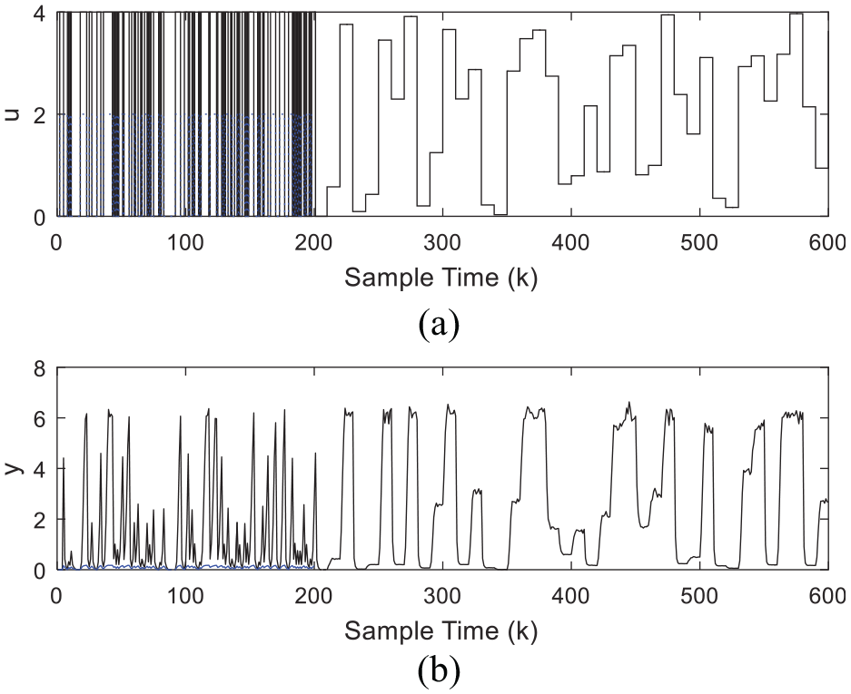
(a) Input signals and (b) output signals.

At first, two sets of binary signals with different sizes of 200 binary signals with 0 or 4 and 200 binary signals with 0 or 2 are employed to learn static output nonlinear block parameter. Set parameters $S_{0} = 0.995$ , $ρ = 1$ , and $λ = 0.03$ , and the number of fuzzy ruler is 14. The estimation of the static output nonlinear block is shown in Figure 6. As can be easily seen from Figure 6, the proposed parameter learning approach can effectively represent the static output nonlinearity of the Hammerstein–Wiener model with disturbance.

Figure 6.

The estimation of the static output nonlinear block.

Next, inputs and corresponding outputs from training samples of binary signals are employed for learning the unknown parameter of the linear block. In this study, we select 5000 binary signals with 0 or 4 for certifying the effectiveness of the correlation analysis method.

From Table 1 and Figure 7, the proposed correlation analysis algorithm can obtain more accurate parameter estimation of dynamic linear block than the RLS algorithm⁴¹ for uncertainty process disturbance. With the increase in noise-to-signal ratio, the proposed learning algorithm has more obvious advantages.

Table 1.

The parameter learning results of dynamic linear block under binary signal.

$δ_{ns}$	k	Correlation analysis algorithm					RLS algorithm⁴¹
		${\hat{b}}_{1}$	${\hat{b}}_{2}$	${\hat{b}}_{3}$	${\hat{b}}_{4}$	$δ$	${\hat{b}}_{1}$	${\hat{b}}_{2}$	${\hat{b}}_{3}$	${\hat{b}}_{4}$	$δ$
$δ_{ns} = 12.14 %$	500	0.8966	0.6144	0.2885	0.0938	0.0175	0.8827	0.5949	0.2674	0.0749	0.0399
	1000	0.8892	0.5964	0.2907	0.1032	0.0133	0.8909	0.5854	0.2724	0.0836	0.0327
	2000	0.9004	0.5917	0.2921	0.1057	0.0114	0.8942	0.5783	0.2728	0.0859	0.0337
	3000	0.9060	0.5947	0.2932	0.1080	0.0117	0.8958	0.5784	0.2730	0.0867	0.0330
	4000	0.9075	0.5965	0.2935	0.1101	0.0130	0.8929	0.5778	0.2733	0.0900	0.0327
	5000	0.9075	0.5959	0.2947	0.1098	0.0125	0.8947	0.5780	0.2744	0.0892	0.0318
$δ_{ns} = 23.37 %$	500	0.8930	0.6235	0.3145	0.0535	0.0484	0.8690	0.5936	0.2826	0.0239	0.0748
	1000	0.8915	0.6236	0.3245	0.0849	0.0339	0.8738	0.5927	0.2843	0.0437	0.0572
	2000	0.9089	0.6174	0.3113	0.0841	0.0246	0.8842	0.5844	0.2713	0.0445	0.0588
	3000	0.9113	0.6186	0.3109	0.0822	0.0267	0.8816	0.5790	0.2725	0.0480	0.0577
	4000	0.9155	0.6189	0.3100	0.0815	0.0286	0.8821	0.5816	0.2705	0.0425	0.0617
	5000	0.9146	0.6162	0.3095	0.0759	0.0301	0.8836	0.5796	0.2708	0.0371	0.0658
True		0.9	0.6	0.3	0.1	0	0.9	0.6	0.3	0.1	0

RLS: recursive least squares.

Figure 7.

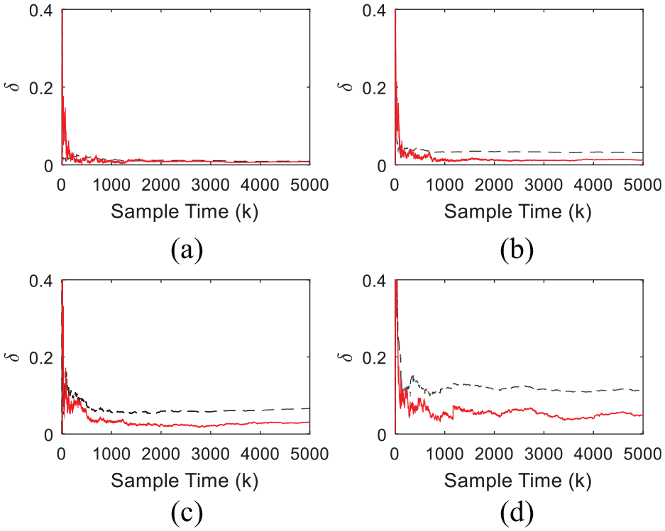
The correlation analysis algorithm (red solid line) and the recursive least squared algorithm (black dashed line):(a) $δ_{ns} = 5.38 %$ , (b) $δ_{ns} = 12.14 %$ , (c) $δ_{ns} = 23.37 %$ , and(d) $δ_{ns} = 33.19 %$ .

Based on the inputs and outputs of the random signal, the parameters of the input static nonlinear block are learned using the design parameters $S_{0} = 0.97$ , $ρ = 1$ , and $λ = 0$ , and the number of fuzzy ruler is 12. Estimation of the input nonlinear block is illustrated in Figure 8. As shown in Figure 8, the proposed model and learning algorithm can effectively simulate static input nonlinearity

Figure 8.

Comparisons of the approximation of the static input nonlinear block.

Finally, to verify the availability of the proposed parameter learning method, the polynomial model–based input nonlinearity is also constructed utilizing the same observed input and output data. The polynomial model is as follows

$\hat{v} (k) = p_{1} u (k) + p_{2} u^{2} (k) + \dots + p_{r} u^{r} (k)$ (46)

where $p_{1}, p_{2}, . . ., p_{r}$ are polynomial model parameters and r is the model order. The error comparisons of two different algorithms are given in Table 2, and it is considered to be the best model when the model order is 11. Figure 8 shows the comparisons of the approximation of the input nonlinear block using the proposed method and the polynomial model.

Table 2.

Errors of various polynomial models and the proposed method.

Algorithms		Mean square error	Maximumerror
Polynomialmodel	Orders
	7	0.0116	0.3713
	8	$1.3 \times 10^{- 3}$	0.0765
	9	$1.0 \times 10^{- 3}$	0.0853
	10	$2.8 \times 10^{- 3}$	0.1356
Proposedmethod		$6.7173 \times 10^{- 4}$	0.0505

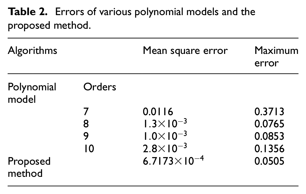
From Table 2 and Figure 8, the proposed parameter learning algorithm has smaller mean square error and maximum error than the polynomial model algorithm. As a result, the proposed parameter learning algorithm can learn well the unknown parameter of the Hammerstein–Wiener model with uncertainty process disturbance.

Case 2

In this case, we take into account the Van de Vusse reaction kinetic process: $A \overset{k_{1}}{\to} B \to^{k_{2}} C, A \overset{k_{3}}{\to} D$ ; the process is implemented in isothermal CSTR. In the Van de Vusse reaction process, the first and second reactions have first-order dynamic characteristics, and the third reaction has second-order dynamic characteristics. The CSTR system is represented by two nonlinear differential equations given by the following equations⁴²

$\begin{matrix} \frac{d C_{A}}{dt} = - k_{1} C_{A} - k_{3} C_{A}^{2} + \frac{F}{V} (C_{Af} - C_{A}) \\ \frac{d C_{B}}{dt} = k_{1} C_{A} - k_{2} C_{B} - \frac{F}{V} C_{B} \end{matrix}$ (47)

where F denotes the inlet flow rate; C_A denotes the concentration of component A; C_B denotes the concentration of component B; C_Af denotes the feed concentration of component A; k₁, k₂, and k₃ denote the kinetic parameters; and V denotes the volume of the reactor. The system parameters of CSTR process are listed in Table 3.

Table 3.

Nominal operating condition and model parameters of CSTR.

Variables	Value (unit)
$k_{1}$	50 h⁻¹
$k_{2}$	100 h⁻¹
$k_{3}$	10 L/mol h
$C_{B 0}$	1.12 mol/L
$C_{A 0}$	3.0 mol/L
$F$	34.3 L/h
$V$	1 L
$C_{Af}$	10 mol/L

CSTR: continuous stirred tank reactor.

The objective of CSTR is to regulate the concentration of component B, C_B, by manipulating the inlet flow rate F. In order to proceed with the proposed learning algorithm, the designed input signals are utilized to achieve system input and output in Figure 9, and the measurable data are normalized by means of $u = (F - 34.3) / 34.3$ and $y = (C_{B} - 1.12) / 1.12$ . Applying the proposed parameter learning algorithm with designed parameters of static input nonlinearity and static output nonlinearity, $S_{0}^{input} = 0.993$ , $ρ^{input} = 1$ , and $λ^{input} = 0.01$ ; $S_{0}^{ioutput} = 0.996$ , $ρ^{o u t p u t} = 1$ , and $λ^{o u t p u t} = 0.01$ ; and the fuzzy rulers of input nonlinearity and output nonlinearity are 9 and 4, respectively.

Figure 9.

The designed input signals of the Hammerstein–Wiener model.

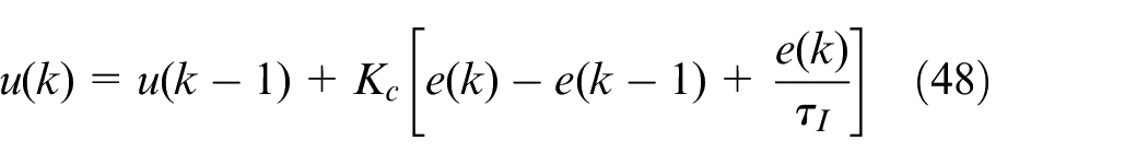
Apply the proposed neuro-fuzzy Hammerstein–Wiener system to the design of controller; the designed control approach of the Hammerstein–Wiener model is shown in Figure 10. The design principle of the Hammerstein–Wiener model is to get rid of input and output nonlinearities and convert the nonlinear Hammerstein–Wiener system into linear system; then the linear system is controlled by the linear controller. In this study, the nonlinear proportional–integral (PI) controller with $K_{c} = 0.5$ and $τ_{I} = 25$ is adopted in the nonlinear control approach. For the sake of contrast, the linear PI controller, as described in equation (48) with $K_{c}^{linear} = 2$ and $τ_{I}^{l i n e a r} = 10$ , is adopted to control the Hammerstein–Wiener model

$u (k) = u (k - 1) + K_{c} [e (k) - e (k - 1) + \frac{e (k)}{τ_{I}}]$ (48)

where $e (k) = y_{r} (k) - z (k)$ indicates the error and $y_{r} (k)$ indicates the set point.

Figure 10.

Nonlinear control system for the Hammerstein–Wiener system.

In Figures 11 and 12, the control performance of the linear PI controller and the nonlinear PI controller is given. According to Figures 11 and 12, it is noticeable that the traditional linear PI controller is unable to achieve good control effectiveness with regard to nonlinear Hammerstein–Wiener model. In particular, it results in a sluggish response when the value of the set point is 0.1. Nevertheless, an oscillatory response is discovered when the value of the set point is −0.5. By comparison, the designed nonlinear PI controller in this paper can effectively balance the sluggish and oscillatory response for positive and negative set points. As a result, the nonlinear PI controller can derive good tracking performance under the nominal operating condition.

Figure 11.

Concentration and flow rate of set point 0.1.

Figure 12.

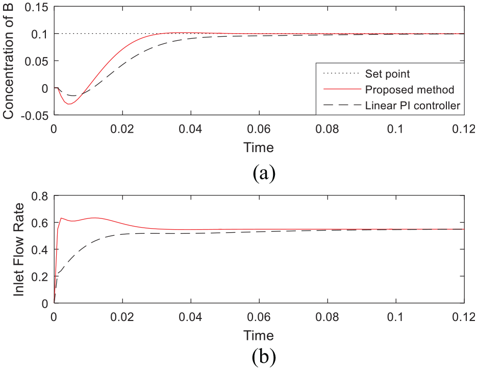
Concentration and flow rate of set point 0.5.

Conclusion

This paper develops a modeling and parameter learning method for the Hammerstein–Wiener model with uncertainty disturbance in which two static nonlinear blocks surround a dynamic linear block. In modeling, two static nonlinearities are represented using independent neuro-fuzzy models, while a dynamic linear block is described using the finite impulse response model. The designed input signals are utilized to analyze the Hammerstein–Wiener model with uncertainty disturbance, resulting in the decoupling of parameter learning of static output nonlinearity, dynamic linear block, and static input nonlinearity. First, the output static nonlinear block parameters can be estimated using two sets of separable signals with different sizes. Moreover, correlation analysis algorithm is developed for learning the parameter of dynamic linear block based on input and output of a set of separable signal. Finally, parameter unbiased estimation of static input nonlinearity block is achieved using least squares method based on input and output of random signal. In numerical cases, two typical Hammerstein–Wiener models are employed to propose the learning algorithm: a discontinuous function and industrial CSTR. The results show that the proposed learning method yields reliable learning results with a high degree of accuracy and those which are minimally affected by disturbance.

Footnotes

Declaration of conflicting interests

The author(s) declared no potential conflicts of interest with respect to the research,authorship,and/or publication of this article.

Funding

The author(s) disclosed receipt of the following financial support for the research,authorship,and/or publication of this article: This work was supported by the Natural Science Foundation of Jiangsu Province under Grant No. BK20191035,Major Basic Research Project of the Natural Science Foundation of the Jiangsu Higher Education Institutions of China under Grant No. 19KJB120002,and the National Natural Science Foundation of China under Grant No. 61773335.

ORCID iD

Feng Li

References

Gao

Shi

, et al. Observer-based fault detection for nonlinear systems with sensor fault and limited communication capacity. IEEE T Automat Contr 2016; 61(9): 2745–2751.

Schindele

Aschemann

Prabel

Nonlinear model-predictive control with hysteresis compensation of an electro-pneumatic clutch for truck applications. Math Comp Model Dyn Syst 2014; 20(2): 105–129.

Shi

Tian

, et al. Modified Volterra model-based non-linear model predictive control of IC engines with real-time simulations. T I Meas Control 2015; 39(2): 208–223.

Jia

Correlation analysis-based error compensation recursive least-square identification method for the Hammerstein model. J Stat Comput Sim 2018; 88(1): 56–74.

Sadeghi

Farrokhi

Block-oriented identification of non-linear systems with input time delay in presence of measurement noise: a Laguerre–neural network approach. T I Meas Control 2018; 41(1): 117–126.

Pouliquen

Pigeon

Gehan

Identification scheme for Hammerstein output error models with bounded noise. IEEE T Automat Contr 2016; 61(2): 550–555.

Chen

Wang

, et al. Recursive identification of Hammerstein systems: convergence rate and asymptotic normality. IEEE T Automat Contr 2017; 62(7): 3277–3292.

Grzegorz

Paweł

Kernel-based identification of Wiener-Hammerstein system. Automatica 2017; 83: 275–281.

Beatriz dos Santos

Elder

Guimaraes

, et al. A Hammerstein-Wiener model for single-electron transistors. IEEE T Electron Dev 2018; 66(2): 1092–1099.

10.

Esmaeilani

Ghaisari

Bagherzadeh

MA.

Bayesian approach to identify Hammerstein-Wiener non-linear model in presence of noise and disturbance. IET Control Theory A 2019; 13(3): 367–376.

11.

Zheng

, et al. A recursive identification algorithm for Wiener nonlinear systems with linear state-space subsystem. Circ Syst Signal Pr 2018; 37: 2374–2393.

12.

Zong

, et al. Parameter estimation of Wiener systems based on the particle swarm iteration and gradient search principle. Circ Syst Signal Pr 2020, https://doi.org/10.1007/s00034-019-01329-1

13.

Liang

Hong

, et al. Neural network modeling and single-neuron proportional-integral-derivative control for hysteresis in piezoelectric actuators. Meas Control 2019; 52(9–10): 1362–1370.

14.

Wang

Cao

Synchronization of delayed neural networks with hybrid coupling via impulsive control. T I Meas Control 2019; 41(13): 3714–3724.

15.

An intelligent machine vision system for detecting surface defects on packing boxes based on support vector machine. Meas Control 2019; 52(7–8): 1102–1110.

16.

Liu

Zhang

Earth pressure balance control of shield tunneling machine based on nonlinear least squares support vector machine model predictive control. Meas Control 2018; 52(1–2): 3–10.

17.

Zhang

Liu

Jiang

, et al. Dissipativity-based resilient asynchronous control for Markov jump systems with sector-bounded nonlinearities. T I Meas Control 2018; 40(9): 2821–2830.

18.

Giri

Bai

EW.

Block-oriented nonlinear system identification: Berlin; Heidelberg: Springer-Verlag, 2010.

19.

Mao

Jia

, et al. Recursive parameter identification of Hammerstein-Wiener systems with measurement noise. Signal Process 2014; 105: 137–147.

20.

Cai

, et al. Double-layered nonlinear model predictive control based on Hammerstein-Wiener model with disturbance rejection. Meas Control 2018; 51(7–8): 260–275.

21.

Jeng

Lin

YW.

Data-driven nonlinear control design using virtual reference feedback tuning based on Block-oriented modeling of nonlinear systems. Ind Eng Chem Res 2018; 57(22): 7583–7599.

22.

Jia

Parameter estimation of Hammerstein-Wiener nonlinear system with noise using special test signals. Neurocomputing 2019; 344: 37–48.

23.

Luo

Song

YD.

Data-driven predictive control of Hammerstein-Wiener systems based on subspace identification. Inform Sciences 2018; 422: 447–461.

24.

Bai

EW.

An optimal two-stage identification algorithm for Hammerstein-Wiener nonlinear systems. Automatica 1998; 34(3): 333–338.

25.

Bai

EW.

A blind approach to the Hammerstein-Wiener model identification. Automatica 2002; 38(6): 967–979.

26.

Crama

Schoukens

Hammerstein-Wiener system estimator initialization. Automatica 2004; 40(9): 1543–1550.

27.

Vörös

Iterative identification of nonlinear dynamic systems with output backlash using three-block cascade models. Nonlinear Dyn 2015; 79: 2187–2195.

28.

Park

Sung

Lee

Modeling of Hammerstein-Wiener processes with special input test signals. Ind Eng Chem Res 2006; 45(3): 1029–1038.

29.

Wills

Schön

Ljung

, et al. Identification of Hammerstein-Wiener models. Automatica 2013; 49(1): 70–81.

30.

Mao

Jia

Recursive identification for Hammerstein-Wiener systems with dead-zone input nonlinearity. J Process Contr 2013; 23: 1108–1115.

31.

Zhang

Hong

Mao

Adaptive control of Hammerstein-Wiener nonlinear systems. Int J Syst Sci 2016; 47(9): 2032–2047.

32.

Zhu

Estimation of an N-L-N Hammerstein-Wiener model. Automatica 2002; 38: 1607–1614.

33.

Wang

Ding

Hierarchical least squares estimation algorithm for Hammerstein-Wiener systems. IEEE Signal Proc Let 2012; 19(12): 825–828.

34.

Mao

Wang

, et al. Identification of Hammerstein-Wiener models based on bias compensation recursive least squares. Acta Automatica Sinica 2010; 36(1): 163–168.

35.

Allafi

Zajic

Uddin

, et al. Parameter estimation of the fractional-order Hammerstein-Wiener model using simplified refined instrumental variable fractional-order continuous time. IET Control Theory A 2017; 11(15): 2591–2598.

36.

Lang

ZQ.

On identification of the controlled plants described by the Hammerstein systems. IEEE T Automat Contr 1994; 39(3): 569–573.

37.

Chen

Wang

JS.

A Hammerstein-Wiener recurrent neural network with frequency-domain eigensystem realization algorithm for unknown system identification. J Univer Comput Sci 2009; 15(13): 2547–2565.

38.

Abouda

Ben Halima Abid

Elloumi

, et al. Identification of nonlinear dynamic systems using fuzzy Hammerstein-Wiener systems. In: Proceedings of the 19th international conference on sciences and techniques of automatic control and computer engineering, Sousse, Tunisia, 24–26 March 2019, pp. 365–370. New York: IEEE.

39.

Jia

Yang

Chiu

MS.

Research on multi-signal based neuro-fuzzy Hammerstein-Wiener model. Acta Automatica Sinica 2013; 39(5): 690–696.

40.

Jia

Peng

Identification method of neuro-fuzzy-based Hammerstein model with coloured noise. IET Control Theory A 2017; 11(17): 3026–3037.

41.

Jia

Yang

Chiu

MS.

Auxiliary model recursive least square algorithm based multi-signal identification of Hammerstein model. J Nanjing U Sci Techno 2014; 38(1): 34–39.

42.

Hahn

Edgar

TF.

A gramian based approach to nonlinearity quantification and model classification. Ind Eng Chem Res 2001; 40(24): 5724–5731.

Modeling and parameter learning method for the Hammerstein–Wiener model with disturbance

Abstract

Keywords

Introduction

The configuration of neuro-fuzzy Hammerstein-Wiener model

The Hammerstein–Wiener model

The neuro-fuzzy Hammerstein–Wiener model

Parameter learning of the neuro-fuzzy Hammerstein–Wiener model

Theorem 1

Learning the static output nonlinear block parameters

Learning the dynamic linear block parameters

Learning the static input nonlinear block parameters

Simulation results and analysis

Case 1

Case 2

Conclusion

Footnotes

Declaration of conflicting interests

Funding

ORCID iD

References