Sage Journals: Discover world-class research

Abstract

This study presents a prediction technique for the output current of a photovoltaic grid-connected system by using random forests technique. Experimental data of a photovoltaic grid-connected system are used to train and validate the proposed model. Three statistical error values, namely root mean square error, mean bias error, and mean absolute percentage error, are used to evaluate the developed model. Moreover, the results of the proposed technique are compared with results obtained from an artificial neural network-based model to show the superiority of the proposed method. Results show that the proposed model accurately predicts the output current of the system. The root mean square error, mean absolute percentage error, and mean bias error values of the proposed method are 2.7482, 8.7151, and −2.5772%, respectively. Moreover, the proposed model is faster than the artificial neural network-based model by 0.0801 s.

Keywords

Modeling of photovoltaic systems random forests artificial neural network performance evaluation

Introduction

In recent years, the installation of photovoltaic (PV) systems has rapidly expanded (Rajkumar et al., 2011). Three types of PV systems are generally used, namely stand-alone PV system, hybrid PV system, and grid-connected PV system. Grid-connected PV systems convert solar radiation into electrical power and inject it directly to the grid without storage (Yang et al., 2010). Grid-connected PV system supports the stability of the electrical power of the system voltage, reduces electrical losses, and reduces the loading level of power transformers (Albuquerque et al., 2010). However, the connection of a PV system to a conventional electrical power system changes the nature of this system from a passive to an active electrical power system (Masters, 2013). Thus, the new nature of the electrical power system must be considered from many viewpoints, such as system’s protection and management. Based on that, grid-connected PV system must be optimally designed, installed, and operated to achieve a secure and stable electrical power system.

The key role of optimally sizing, installing, and controlling a grid-connected PV system is represented by predicting system’s output power or current (Milosavljević et al., 2015). The output current of a grid-connected PV system is a function of meteorological variables, such as solar radiation and ambient temperature. Therefore, any PV system performance model is usually developed based on these meteorological variables (Sharma and Chandel, 2013).

In general, several methods for predicating PV systems output current can be found in the literature (Almonacid et al., 2009, 2014; Bacher et al., 2009; Bahgat et al., 2005; Blair et al., 2008; Chen et al., 2005; Chow et al., 2012; Chowdhury and Rahman, 1988; Ding et al., 2011; Eke and Demircan, 2013; Grimaccia et al., 2011; Hiyama and Kitabayashi, 1997; Kermanshahi and Iwamiya, 2002; Rus-Casas et al., 2014). These methods can be classified as linear models (Bacher et al., 2009), auto-regression integrated moving average models and ARMA models (Chowdhury and Rahman, 1988), fuzzy logic models (Grimaccia et al., 2011), and artificial neural network (ANN)-based models (Almonacid et al., 2014). However, the accuracy of some of these models such as linear, ARMA, and fuzzy logic models is questionable, particularly when dealing with a highly uncertain energy source such as the Sun (Blair et al., 2008; Eke and Demircan, 2013).

By contrast, ANNs, as an alternative to the aforementioned models, have been successfully employed for this purpose and are capable of handling the uncertainty issues of solar radiation (Almonacid et al., 2009; Chow et al., 2012; Ding et al., 2011). In Hiyama and Kitabayashi (1997), the ANN technique was used to predict the output power of a PV system. Multilayer perceptron feedforward neural networks were used for this purpose. The network inputs were solar radiation, temperature, and wind velocity. The error in predicting the system output power was in the range of 7.7–17.6%. Similar studies were presented in Bahgat et al. (2005), Chen et al. (2005), Kermanshahi and Iwamiya (2002), and Rus-Casas et al. (2014). According to these studies, the most recommended neural network is the feedforward ANN, whereas the most recommended factors for predicting system output power or current are solar radiation and ambient temperature. The prediction error of system’s output power or current is in the range of 5–11%. In Sulaiman et al. (2012), a hybrid multilayer feedforward neural network is used for predicting the output power of a grid-connected PV system. The solar radiation and PV module’s temperature are utilized as input variables while the energy generated by the system was the output of this model. In Lo Brano et al. (2014), an adaptive approach based on different topologies of ANNs is proposed for modeling the output power of a grid-connected PV system. The output power is obtained using three different types of ANNs, namely one hidden layer multilayer perceptron, a recursive neural network, and a gamma memory trained with the back propagation. Experimental data containing solar radiation, air temperature, and wind speed were utilized for the training stage. In addition, the training was carried out with historical output power data available for two PV modules. The performance of these models was compared with actual performance. Based on the results, the best adopted methodology for output power forecasting is selected. In Almonacid et al. (2014), a predicting methodology for forecasting the PV output power for 1 h ahead has been developed. Hourly solar global radiation and air temperature data were utilized for developing the model. Here, two ANN models were developed to predict the solar global radiation and air temperature in the next hour.

Based on that ANNs have been used widely for predicting PV systems output. However, the use of ANNs for such a purpose has some limitations and challenges such as the complexity of the training process, the calculation of the hidden layer neurons, and the ability of handling highly uncertain data (Khatib et al., 2012). In the meanwhile, some novel methods with high accuracy and capability of handling highly uncertain data, such as random forests (RFs), can be used for this purpose.

RFs are an ensemble machine learning method that uses many decision tree models for classification and regression. RFs are a combination of tree predictors that depend on the random vector values independently at the same distribution in the forest (Breiman, 2001). The tree construction in the RFs does not depend on the previous trees. The trees are created independently by using bootstrap aggregation of the dataset (Breiman, 1996). RFs do not over fit as a predictor and run fast and efficiently when handling large datasets which gives it a superior predictive performance. Furthermore, RFs do not require assumptions of data distribution through the trees. Moreover, RFs can handle both continuous and discrete variables (Tooke et al., 2014).

The RFs technique was successfully used for modeling the solar radiation. In Sun et al. (2016), the authors used the RFs model for predicting daily solar radiation for three sites in China. The default number of the parameters was used (500 trees and five leaves per tree). The results of this research work show that the performance of the RFs model is better than the results obtained by linear, exponential, and logarithmic models. In the meanwhile, in Kratzenberg et al. (2015), the authors used the RFs model for predicting hourly and the daily solar radiation. Here, the internal RFs parameters were not mentioned. In Gala et al. (2015), RF-based model with different values of the internal RFs parameters to predict hourly solar radiation is presented. The authors set the number of trees in the range of (10, 50, 100, and 300 trees), while the range of leaves is proposed to be five and 20 leaves per tree. Here, the best number of trees and leaves per tree are selected based on the best performance of the model.

This study presents a technique for predicting the output current of a PV grid-connected system by using RFs. Experimental data of a 3 kWp PV grid-connected system installed at the Universiti Kebangsaan Malaysia campus are used. These data contain hourly solar radiation, ambient temperature, and actual system output current. The performance of the developed RFs model is compared with that of an ANN-based model to show the superiority of the proposed method.

Mathematical modeling of PV current

In general, each PV module consists of a number of solar cells that are connected in series and parallel. In the dark (with no sunlight), the solar cell acts as a diode in reverse mode. Under solar radiation, the solar cell generates DC current. A solar cell can be represented as an electrical circuit, as depicted in Figure 1.

Figure 1.

Solar cell equivalent electrical circuit.

Equation (1) represents the behavior of the solar cell $\begin{matrix} I = I_{ph} - I_{0} {e^{\frac{q (V + {IR}_{s})}{mkT}} - 1} - \frac{V + {IR}_{s}}{R_{sh}} \end{matrix}$ (1)

where $R_{s}$ is a resistance that represents the semiconductor material losses, $R_{sh}$ represents the leakages current, $I_{ph}$ is the photogenerated current, $I_{0}$ is the saturation current, $T_{c}$ is the cell absolute temperature, $k$ is the Boltzmann constant, $m$ is the diode ideality factor, and $q$ is the electrical charge (Masters, 2013). Therefore, $R_{s}$ is usually estimated by this ratio $R_{s} = [1 - \frac{FF}{{FF}_{0}}] (\frac{V_{oc}, STC}{I_{sc}, STC})$ (2)

where STC is the standard test condition wherein solar radiation (G) is 1000° w/m², ambient temperature (T_A) is 25℃, and wind speed (v_w) is 1.5 m/s. V_oc is the open-circuit voltage, I_sc is the short-circuit current, FF is the actual fill factor, and FF₀ is the ideal fill factor of the solar cell at R_s=0. FF₀ can be calculated by the following ${FF}_{0} = \frac{V_{0} - Ln (V_{0} + 0.72)}{V_{0}}$ (3)

where ( $V_{0})$ is the ratio between the open-circuit voltage and thermodynamic voltage ( $VT$ ). The output current of a solar cell can be described theoretically as a linear regression $I = I_{STC} (\frac{G}{G_{STC}}) [1 + α (T_{c} - T_{c, STC})]$ (4)

where $I_{STC}$ is the PV module current at STC, $G$ is the solar radiation, $G_{STC}$ is the solar radiation under STC, $α$ is the short-circuit temperature coefficient, and $T_{c, STC}$ is the cell temperature at STC. The cell temperature ( $T_{c}$ ) can be obtained from the ambient temperature ( $T_{A}$ ), and the nominal operating temperature of the cell ( $NOCT$ ) which is usually supplied by the manufacturer. $NOCT$ is defined as the operating temperature of a PV module under solar radiation ( $G$ ) of 800° w/m², ambient temperature ( $T_{A}$ ) of 20℃, and wind speed ( $v_{w}$ ) of 1 m/s (Masters, 2013). $T_{c}$ can be calculated by the following $T_{c} = T_{A} + (\frac{NOCT - 2 0^{\circ}}{800}) * G$ (5)

RFs technique

The RFs model implies bagging and random decision trees. Bagging can be defined as a technique that is applied for prediction functions so as to reduce the variance of such functions. RFs, therefore, are an extension of bagging that use decorrelated trees. In general, a simple RFs model is usually developed by using low number of input variables so as to have them splitted randomly at each node (Breiman and Cutler, 2014).

RF-based prediction models’ development procedure usually starts by establishing a new set of values that are equal to the size of the originally spotted data. These data are selected from the original dataset by a random bootstrapping. After that, the selected dataset is formulated as a sequence of binary splits so as to create the desired decision trees. Here, at each node of these trees, the split is calculated by selecting the value of the variable subject to a minimum error rate. Eventually, an average of the aggregating predictors is taken for regression prediction and while the majority vote is taken for prediction in classification (Liaw and Wiener, 2002).

Bootstrap aggregation techniques facilitate the determination of error and the rate of change of the input on the output variables (variable importance (VI)) (Breiman, 2001). The accuracy of this process (Error rates) and variables correlation (variables importance) are calculated by omitting values from each bootstrap sample in a process called “out-of-bag” (OOB) data (Breiman, 2001; MATLAB, 2016). OOB data have an important role in tree growth process, whereas OOB data are compared with the predicted values at each step.

Classification and regression

Classification and regression trees are a recursive partitioning method that is used for predicting continuous dependent variables in regression and categorical predictor variables in classification. The decision follows the flow of the nodes from the root to the leaf for all the trees in forest that contains the response. In regression trees, the response has resulted in a numeric form, while it is resulted in a nominal form (true or false) in classification trees.

On one hand, classification trees are used in which objects are recognized, understood, and differentiated (Alpaydin, 2010). Classification trees, in general, group the objects into independent categories based on a specific criterion. The main role of the classification trees is to provide an understanding on the relationships between the subjects and the objects. Classification trees are mostly used in language, inference, decision making, and in all types of environmental interaction. The principle of classification trees is overlapped with the machine learning role (Mills, 2011).

On the other hand, regression trees are a statistical method that is used for determining the relationships between the variables. Many techniques for modeling and analysing the data are included in regression when the relationships are studied between a dependent variable and one or more independent variables (Armstrong, 2012). Regression trees are widely used in prediction, and its role overlaps with the field of machine learning as in the classification trees.

The principle of the RFs is changed depending on the constructed regression and classification trees (Liaw and Wiener, 2002). In general, the decision trees are constructed based on the following phases. First, all training input data are used to examine all the possibilities of the binary split in each predictor or classifier, then the split that has the best optimization criterion is chosen. The optimization criterion in regression trees denotes that the chosen split has the minimum mean square error (MSE) which is calculated between the predicted data and the actual data during the training process. In classification trees, one of three measures including Gini’s diversity index, deviance, or twoing rule is used to choose the split. Second, the selected split is imposed to divide into two new child nodes. Finally, the process is repeated for new child nodes until finishing the construction of the trees (reach the minimum MSE in regression trees) (MATLAB, 2016). In RFs, regression trees are formed by growing each tree depending on a random vector. The RFs predictor is formed by taking the average of all the trees in the forest (Breiman, 2001).

RFs algorithm

The procedure for predicting the response in RFs algorithm is a combination between training and testing phases. In the training phase, the RFs algorithm starts by drawing multiple bootstrap samples (N) from the original data and then creates a number of unpruned classification or regression trees (CART) for each N. About one-third of the samples are left out in the construction which are called OBB data (Liaw and Wiener, 2002). The OOB data is a term used to get a running unbiased estimate of the prediction error as trees are added to the forest in the construction phase. Thus, OOB data play a primary role in tree growth, that is, OOB data is compared with the predicted values at each step. Meanwhile, the trees are constructed into the forest according to minimize the error rate than the obtained value of the OOB data (Breiman, 2001). The RFs error rate of Breiman (2001) depends on two parameters: the correlation between any two trees and the strength of each tree individually. After creating the final splits, the data are predicted at each bootstrap iteration by using the tree growth technique with the bootstrap sample (Liaw and Wiener, 2002). Based on that, the number of trees in the forest is a hyper-parameter in the RFs algorithm which should be found so as to assure accurate prediction results. Breiman (2001) suggests trying the default, half of the default, and twice the default and then taking the best one.

In testing phase, the testing data are distributed in the forest to start the prediction procedure. The data flow into the trees is traced to the constructed splits. The final nodes are predicted in the new data by determining the average aggregation of the predictors through all trees. Figure 2 shows the main structure of the RFs algorithm.

Figure 2.

Structure of the RFs algorithm. RF: random forest.

VI measure

RFs algorithm provides a significant measure of the VI into the dataset. This measure is implemented into the training phase which has examined the individual effects of each of the inputs variables on the output of the algorithm. The VI aim is to improve the prediction accuracy (the VI value decreases when the prediction accuracy increases) which is done using the OOB data and during the dawning of the N in each tree by sampling with replacement (Breiman, 2001).

The VI of any variable can be obtained by randomly altering all the values of the variables (f) in the OOB sample in each tree into the forest. The VI measure is calculated as ratio of the average of the difference between the prediction accuracy before and after altering the variable f to the total number of all the trees into the forest (Breiman, 2001). The importance score of each variable is obtained by using the following equation (Guo et al., 2011) $\begin{matrix} {VI}^{(t)} (f) = \frac{\sum_{T} (\frac{\sum_{x_{i} \in β^{c (t)}} I (L_{j} = c_{i}^{(t)})}{| β^{c (t)} |} - \frac{\sum_{x_{i} \in β^{c (t)}} I (L_{j} = c_{i, π f}^{(t)})}{| β^{c (t)} |})}{T} \end{matrix}$ (6)

where $β^{c (t)}$ corresponds to OBB samples for a specific tree, $β^{(t)}$ represents the in-bag samples for a particular tree, t represents the tree number (1, 2, … , T), T is the total number of trees, and $c_{i}^{(t)}$ and $c_{i, π f}^{(t)}$ are the predicted classes for each sample for a tree before and after altering the variable. x_i represents the sample value, and L_j is the true label; both are in the training stage.

Application of the RFs technique for predicting the PV output current

Figure 3 shows the RFs prediction flowchart. The prediction of a PV system output current starts by first setting the input samples and variables into the Bagger algorithm. In this work, the inputs are solar radiation, ambient temperature, day number, hour, latitude, longitude, and number of PV modules. As a fact, no mathematical formula sets the optimum number of trees (Liaw and Wiener, 2002). In this application, the initial number of trees is supposed to be 250 trees as the half of the default number of tress as Breiman (2001) suggested, and the initial number of leaves in each tree is supposed to be five as the default of the Bagger algorithm (MATLAB, 2016). In some studies such as Tooke et al. (2014), the authors set the number of trees to 500 during the training and testing phases. Meanwhile, the authors do not optimize the number of trees and leaves, thus affecting system accuracy.

Figure 3.

RFs prediction flowchart. RF: random forest.

The initial numbers implemented in the first stage of the training process of the algorithm are used only to estimate the VI, outliers, and proximity matrix to manage the algorithm parameters. Thereafter, the process for the VI measure is conducted (Ibrahim and Khatib, 2017). As a result, solar radiation, day number, hour, and ambient temperature are the most important variables. However, the other variables are neglected because they have constant values. Thus, the other variables do not affect the prediction process and system accuracy.

Second, the outliers in the training dataset are detected by using cluster analysis. The cluster analysis of data or clustering is a task of grouping the training data in such way that the dataset is in the same group that is more similar to one another than the other groups. Many typical of clustering models are used as subspace models, connectivity models, connectivity models, centroid models, density models, group models, centroid models, distribution models, and graph-based models. In this study, the density model is used. The density model defines the clusters as connected dense regions in the dataset space. The data points in the x-axis are processed by optics and those in the y-axis are processed by the reachability distance. Figure 4 shows that the points that are belonging to a cluster have low reachability distance to their nearest neighbor. Therefore, the model can easily detect clusters of points and noise points that do not belong to any of these clusters. In the RFs algorithm, the outliers are detected by using cluster analysis.

Figure 4.

Cluster analysis for the training dataset.

However, in machine learning techniques, removing the outliers data from the dataset will significantly increase the accuracy of the results. Here, the outliers in the training dataset are detected, removed, replaced. Outlier detection is the identification of observations that do not conform to a prospective pattern in a dataset. It is normally accomplished with statistics and thresholds. Cluster analysis is one of the most popular technique for detecting outliers or noises that do not belong to a dataset. A normal distribution model is used to analyze the dataset. The outliers expected in the dataset are depicted in Figure 5, which shows the percentage of training dataset detected to be outliers. These percentages are 54.4% of the dataset found in the first pattern, 0.265% in the second pattern, 0% in the third pattern, 0.53% in the fourth pattern, 1.6% in the fifth pattern, 4.51% in the sixth pattern, 11.6% in the seventh pattern, 18.03% in the eighth pattern, and 9.02% in the ninth pattern. However, the algorithm is developed to remove these outliers and replace them by using a better way to increase the accuracy of the results.

Figure 5.

Outlier measure in the training dataset.

Finally, the optimization of the number of trees and the number of leaves in each tree for the modified dataset and greatest VI is conducted. In this stage, an iterative method starts the training phase for large trial numbers; these trial numbers are 50,000 values for 500 trees and 100 leaves to find the best number of trees and leaves in each tree.

Proposed model evaluation

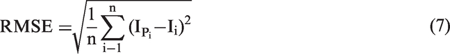
In this paper, three values are used to evaluate the proposed model. They are root MSE (RMSE), mean absolute percentage error (MAPE), and mean bias error (MBE). RMSE is an efficiency indicator of the prediction process; a large positive RMSE value represents a large deviation scale in the prediction values from the target values. MBE or mean forecasted error is used as an average deviation indicator; a negative value means that the prediction is underforecasted and vice versa. MAPE represents an accuracy indicator. RMSE, MBE, and MAPE are expressed as follows (Ibrahim et al., 2017) $\begin{matrix} RMSE = \sqrt{\frac{1}{n} \sum_{i - 1}^{n} {(I}_{P_{i}} {- I}_{i})^{2}} \end{matrix}$ (7) $\begin{matrix} MAPE = \frac{1}{n} \sum_{i = 1}^{n} | \frac{I_{i} - I_{P_{i}}}{I_{i}} | \end{matrix}$ (8) $\begin{matrix} MBE = \frac{1}{n} \sum_{i = 1}^{n} I_{P_{i}} - I_{i} \end{matrix}$ (9)

where $I_{P_{i}}$ represents the predicted value, I_i is the target value, and n is the number of observations.

Results and discussion

In this research, the output current of a 3 kWp PV system installed at the Faculty of Engineering Built & Environment, UKM, Malaysia (101.7713° E, 2.921065° N) is used (see Figure 6). The system consists of polycrystalline silicon panels (25 modules) tilted at 15°. The specifications of the PV module are listed in Table 1.

Figure 6.

Utilized dataset profile.

Table 1.

Electrical characteristics of PV module at STC.

Module type	STF-120P6
Rated power ( $P_{max})$	120 W
Open-circuit voltage ( $V_{oc}$ )	21.5 V
Short-circuit current ( $I_{sc}$ )	7.63 A
Voltage at MPP ( $V_{MP}$ )	17.4 V
Current at MPP ( $I_{MP}$ )	6.89 A
Nominal operation cell temperature ( $NOCT$ )	43.6℃
Temperature coefficient of $I_{sc}$ (α)	6.93 mA%/℃
Temperature coefficient of $V_{oc}$ (β)	−0.068 V/℃
Temperature Coefficient of $P_{max}$ (γ)	−0.39 $%$
Dimension of module	1470 mm × 662 mm × 45 mm

PV: photovoltaic; STC: standard test condition.

The performance data of the system, as well as meteorological data (solar radiation and ambient temperature), are used in this research. Six months of the hourly recorded data are utilized in the research work. The monitoring system consists of solar radiation transmitter of high-stability silicon PV detector model WE300 with accuracy of ± 1%, temperature sensor for the surface of the PV panel model WE710 with accuracy of ±0.25℃, air temperature sensor model WE700 with range of −50℃ to + 50℃ and accuracy of ± 0.1℃, and current transducer Model: CTH-050 with input range of 0–50 A (DC) and output of 4–20 mA. In this research, the dataset used is divided into two parts: 70% for training and 30% for testing and validation. Figure 7 shows the dataset utilized in this research.

Figure 7.

Capture of the testing system.

Figure 8 shows the VI rates for the seven inputs used in this study. From Figure 6, the most important variable is solar radiation with a rate of 2.4 out of 2.5. Then, day number has a rate of 0.87 out of 2.5, whereas hour has a rate of 0.77 out of 2.5. Finally, ambient temperature has a rate of 0.6 out of 2.5. The other inputs have a rate of 0 out of 2.5, that is, these variables have no effect on the predicted values of the output current. Following these results, the inputs that were used in this study are solar radiation, ambient temperature, day number, and hour.

Figure 8.

Variable importance measure.

Optimizing the parameters of the RFs prediction algorithm requires searching for the best number of trees and the number of leaves in each tree that achieve the best values of RMSE, MAPE, and MBE. Tables 2 to 4 show the 5000 trials for 500 trees with 100 leaves in each tree and the effect of the numbers of trees and leaves on prediction accuracy. From the tables, the best number of trees is found to be 65, whereas the best number of leaves is found to be one leaf per tree.

Table 2.

RMSE values for 50,000 probabilities. The bold values identify the best numbers of trees and leaves.

$NTrees / NTreesNLeavesNLeaves$	1	2	..	50	..	99	100
1	0.070574	0.065317	..	0.201384	..	0.239002	0.120607
2	0.070890	0.044500	..	0.084257	..	0.115759	0.120174
:	:	:	:	:	:	:	:
65	0.030707	0.033739	..	0.057588	..	0.074859	0.078639
:	:	:	:	:	:	:	:
499	0.032637	0.032829	..	0.053879	..	0.0793581	0.084467
500	0.032873	0.033188	..	0.054036	..	0.0797012	0.076904

RMSE: root MSE.

Table 3.

MAPE values for 50,000 probabilities. The bold values identify the best numbers of trees and leaves.

$NTrees / NTreesNLeavesNLeaves$	1	2	..	50	..	99	100
1	12.67039	11.93032	..	20.243	..	22.10267	16.34645
2	12.75921	10.23325	..	13.62276	..	17.00787	15.83865
:	:	:	:	:	:	:	:
65	8.715075	9.104025	..	11.40975	..	13.28555	13.74957
:	:	:	:	:	:	:	:
499	9.025179	9.052338	..	11.30994	..	13.59797	14.03981
500	9.199654	9.086893	..	11.32157	..	13.69799	13.41354

MAPE: mean absolute percentage error.

Table 4.

MBE values for 50,000 probabilities. The bold values identify the best numbers of trees and leaves.

$NTrees / NTreesNLeavesNLeaves$	1	2	..	50	..	99	100
1	−0.05955	−0.00171	..	−0.03952	..	0.060048	0.010962
2	−0.05598	−0.01938	..	0.06463	..	0.021265	0.026504
:	:	:	:	:	:	:	:
65	−0.0288	−0.03167	..	0.04840	..	0.074859	0.078639
:	:	:	:	:	:	:	:
499	−0.03587	−0.03277	..	−0.00456	..	0.023408	0.026086
500	−0.03832	−0.03375	..	−0.09834	..	0.023997	0.023575

MBE: mean bias error.

After setting the parameters of the algorithm, the training process was conducted by using 70% of the dataset. Thereafter, 30% of these data are used to validate the proposed model. Actual data, as well as the predicted data by the ANN-based model, are compared with the predicted data by the proposed RFs model to show the superiority of the proposed model. Figure 9 shows the PV system output current based on the developed RFs model, ANN-based model, and actual data. From the figure, the developed RFs model shows better results than the ANN-based model. Moreover, the predicted values by RFs do not deviate from the interval of the measured values. Furthermore, the RF-based model is faster than the ANN-based model in terms of training and testing processes. Table 5 shows the evaluation of the proposed models. From Table 5, RFs exceed the ANN in predicting the system output current. The RMSE, MAPE, and MBE values for the proposed model are 2.7, 8.7, and −2.58%, respectively. These results prove the superiority of RFs in predicting the system output current compared with the ANN-based model.

Figure 9.

PV output current by ANN-based model and RFs model through 72 h. ANN: artificial neural network; PV: photovoltaic; RF: random forest.

Table 5.

Statistical values and time consumption of methodologies in PV output current prediction.

Model	RMSE (A)	RMSE (%)	MAPE (%)	MBE (A)	MBE (%)	Cons. time (s)
ANN	0.0321	2.9392	10.3743	−0.0292	−2.5912	0.4847
RFs	0.0307	2.7482	8.7151	−0.0288	−2.5772	0.4046

ANN: artificial neural network; MAPE: mean absolute percentage error; MBE: mean bias error; PV: photovoltaic; RF: random forest; RMSE: root MSE.

Conclusion

A model for predicting the output current of a PV system by using RFs was presented in this paper. Experimental data of a 3 kWp PV system were used in developing the proposed model. Three statistical error values, namely RMSE, MAPE, and MBE, were employed to evaluate the accuracy of the proposed model. Based on the results, the RFs model was found to be accurate in modeling PV output current and exceeded the ANN-based model. The RMSE, MAPE, and MBE values for the proposed RFs model were 2.7482, 8.7151, and −2.5772%, respectively. Based on that, the proposed RFs model can therefore be used as an efficient machine learning for predicting hourly output current of PV system.

Footnotes

Declaration of conflicting interests

The author(s) declared no potential conflicts of interest with respect to the research,authorship,and/or publication of this article.

Funding

The author(s) disclosed receipt of the following financial support for the research,authorship,and/or publication of this article: The authors would like to acknowledge the financial support from the Universiti Kebangsaan Malaysia funding under the research projects ETP-2013-044 and DIP-2014-028. Financial support is also received from Alpen-Adria-Universität Klagenfurt Project Number AST4340004 (Smart Grids).

References

Albuquerque

Moraes

Guimarães

et al. (2010) Photovoltaic solar system connected to the electric power grid operating as active power generator and reactive power compensator. Solar Energy 84: 1310–1317.

Almonacid

Pérez-Higueras

Fernández

et al. (2014) A methodology based on dynamic artificial neural network for short-term forecasting of the power output of a PV generator. Energy Conversion and Management 85: 389–398.

Almonacid

Rus

Pérez

et al. (2009) Estimation of the energy of a PV generator using artificial neural network. Renewable Energy 34: 2743–2750.

Alpaydin E (2010) Introduction to machine learning. In: Dietterich T (ed.) Adaptive Computation and Machine Learning Series. 2nd ed. Cambridge, USA: MIT Press, pp.17–161. Available at: http://mitpress.mit.edu/books/introduction-machine-learning.

Armstrong

(2012) Illusions in regression analysis. International Journal of Forecasting 28(3): 689–694.

Bacher

Madsen

Nielsen

(2009) Online short-term solar power forecasting. Solar Energy 83(10): 1772–1783.

Bahgat

ABG

Helwa

Ahmad

et al. (2005) Maximum power point tracking controller for PV systems using neural networks. Renewable Energy 30: 1257–1268.

Blair N, Mehos M, Christensen C, et al. (2008) Modeling photovoltaic and concentrating solar power trough performance, cost, and financing with the solar advisor model: Preprint. In: 37th annual conference of American Solar Energy Society (ASES), National Renewable Energy Laboratory, San Diego, California, USA, pp. 1–7. Available at: https://www.osti.gov/scitech/biblio/928609 (accessed 16 September 2016).

Blair

Mehos

Christensen

et al. (2008) Modeling photovoltaic and concentrating solar power trough performance, cost, and financing with the solar advisor model preprint. Solar Energy, 1–7.

10.

Breiman

(1996) Bagging predictors. Machine Learning 24: 123–140.

11.

Breiman

(2001) Random forests. Machine Learning 45: 5–32.

12.

Breiman L and Cutler A (2014) Random forests. 2004. Available at: http://www.stat.berkeley.edu/∼breiman/RandomForests/cchome.htm (accessed 10 July 2016).

13.

Chen

Yang

Dong

et al. (2005) Time-series forecasting using flexible neural tree model. Information Sciences 174(3–4): 219–235.

14.

Chow

SKH

Lee

EWM

DHW

(2012) Short-term prediction of photovoltaic energy generation by intelligent approach. Energy and Buildings 55: 660–667.

15.

Chowdhury

Rahman

(1988) Is central station photovoltaic power dispatchable? IEEE Transactions on Energy Conversion 3(4): 747–754.

16.

Ding

Wang

(2011) An ANN-based approach for forecasting the power output of photovoltaic system. Procedia Environmental Sciences 11: 1308–1315.

17.

Eke

Demircan

(2013) Performance analysis of a multi crystalline Si photovoltaic module under Mugla climatic conditions in Turkey. Energy Conversion and Management 65: 580–586.

18.

Gala

Fernández

Díaz

et al. (2015) Hybrid machine learning forecasting of solar radiation values. Neurocomputing 176: 1–12.

19.

Grimaccia F, Mussetta M and Zich R (2011) Neuro-fuzzy predictive model for PV energy production based on weather forecast. In: Proceedings of the IEEE international conference on fuzzy systems (FUZZ 2011), IEEE, Taipei, Taiwan, pp.2454–2457. Available at: http://ieeexplore.ieee.org/document/6007687/ (accessed 20 September 2016).

20.

Guo

Chehata

Mallet

et al. (2011) Relevance of airborne lidar and multispectral image data for urban scene classification using Random Forests. ISPRS Journal of Photogrammetry and Remote Sensing 66(1): 56–66.

21.

Hiyama

Kitabayashi

(1997) Neural network based estimation of maximum power generation from PV module using environmental information. IEEE Transactions on Energy Conversion 12(3): 241–247.

22.

Ibrahim

Khatib

(2017) A novel hybrid model for hourly global solar radiation prediction using random forests technique and firefly algorithm. Energy Conversion and Management 138: 413–425.

23.

Ibrahim

Khatib

Mohamed

(2017) Optimal sizing of standalone photovoltaic system for remote housing electrification using numerical algorithm and improved system models. Energy 126: 392–403.

24.

Kermanshahi

Iwamiya

(2002) Up to year 2020 load forecasting using neural nets. International Journal of Electrical Power & Energy Systems 24: 789–797.

25.

Khatib

Mohamed

Sopian

(2012) A review of solar energy modeling techniques. Renewable and Sustainable Energy Reviews 16(5): 2864–2869.

26.

Kratzenberg

Helmut

Preede

et al. (2015) Identification and handling of critical irradiance forecast errors using a random forest scheme – A case study for southern Brazil. Energy Procedia 76(1876): 207–215.

27.

Liaw

Wiener

(2002) Classification and regression by random forest. R News 2(3): 18–22.

28.

Lo Brano

Ciulla

Di Falco

(2014) Artificial neural networks to predict the power output of a PV panel. International Journal of Photoenergy 2014: 12.

29.

Masters

(2013) Renewable and Efficient Electric Power Systems, 2nd ed. Hoboken, NJ: John Wiley & Sons, Inc.

30.

MATLAB (2016) (2016) TreeBagger. mathworks. Available at: http://www.mathworks.com/help/stats/treebagger.html (accessed 28 August 2016).

31.

Mills

(2011) Efficient statistical classification of satellite measurements. International Journal of Remote Sensing 32(21): 6109–6132.

32.

Milosavljević

Pavlović

Piršl

(2015) Performance analysis of a grid-connected solar PV plant in Niš, Republic of Serbia. Renewable and Sustainable Energy Reviews 44: 423–435.

33.

Rajkumar

Ramachandaramurthy

Yong

et al. (2011) Techno-economical optimization of hybrid PV/wind/battery system using neuro-fuzzy. Energy 36(8): 5148–5153.

34.

Rus-Casas

Aguilar

Rodrigo

et al. (2014) Classification of methods for annual energy harvesting calculations of photovoltaic generators. Energy Conversion and Management 78: 527–536.

35.

Sharma

Chandel

(2013) Performance and degradation analysis for long term reliability of solar photovoltaic systems: A review. Renewable and Sustainable Energy Reviews 27: 753–767.

36.

Sulaiman

Khawa

Musirin

et al. (2012) An artificial immune-based hybrid multi-layer feedforward neural network for predicting grid-connected photovoltaic system output. Energy Procedia 14: 260–264.

37.

Sun

Gui

Yan

et al. (2016) Assessing the potential of random forest method for estimating solar radiation using air pollution index. Energy Conversion and Management Journal 119: 121–129.

38.

Tooke

Coops

Webster

(2014) Predicting building ages from LiDAR data with random forests for building energy modeling. Energy and Buildings 68: 603–610.

39.

Yang

Zhao

et al. (2010) Design and analysis of a grid-connected photovoltaic power system. IEEE Transactions on Power Electronics 25: 992–1000.

Modeling of the output current of a photovoltaic grid-connected system using random forests technique

Abstract

Keywords

Introduction

Mathematical modeling of PV current

RFs technique

Classification and regression

RFs algorithm

VI measure

Application of the RFs technique for predicting the PV output current

Proposed model evaluation

Results and discussion

Conclusion

Footnotes

Declaration of conflicting interests

Funding

References