Sage Journals: Discover world-class research

Abstract

Wireline logging plays a critical role in coalbed methane exploration. However, the lack of crucial log data, such as neutron and sonic logs, makes coalbed methane exploration difficult. In this paper, we propose a principal component regression model incorporating a multiscale wavelet analysis, a histogram calibration, a principal component analysis, and a multivariate regression to reconstruct essential neutron and sonic logs from conventional logs (i.e., density, resistivity, gamma ray, spontaneous potential, and caliper logs). Our proposed model does not need core-related correlation, and there is no local optimization. We have applied the model to evaluate coalbed methane content in a real case. Firstly, we use the multiscale wavelet analysis and histogram calibration to improve logs’ reliability and lateral comparability. Then, we apply principal component analysis to transform the well-correlated wireline logs into linearly independent components and regress reconstruction functions for neutron and sonic logs with multivariate regression. The reconstructed logs are like the measured logs in trend, mean, and scale. Finally, we apply the reconstructed neutron logs to predict the coalbed methane-content distribution. The predicted distribution is not only following the regional distribution characteristics of coalbed methane enrichment zones but also validated by the coalbed methane production data. In summary, the successful applications of wireline-log reconstruction and regional coalbed methane-content prediction have demonstrated the reliability of the proposed principal component regression model.

Keywords

Coalbed methane wireline log denoising reconstruction principal component analysis multivariate regression

Introduction

With the advancement of coalbed methane (CBM) exploration and development in China, wireline-logging technologies played a crucial role in CBM reservoir evaluation and development (Chen et al., 2018; Hatherly et al., 2016; Huang et al., 2019; Ren et al., 2018; Teng et al., 2015; Wang et al., 2017; Zhou and Esterle, 2008; Zhou and O’Brien, 2016). However, several factors, such as instrument inconsistency and logging environments, affect log data quality and cause systematic or non-systematic errors (Kang et al., 2018; Koizumi, 2007; Niebuhr et al., 2001). The lack of enough wireline-log data is a common phenomenon in the early stage of CBM exploration. In a given CBM block, most wells have conventional wireline logs, such as density, resistivity, gamma ray, caliper, and spontaneous potential (SP) logs, and only a few boreholes have the neutron and sonic logs. The lack of neutron and sonic logs makes CBM interpretation and evaluation difficult. Therefore, it is desirable to reconstruct neutron and sonic logs using conventional wireline logs.

In the literature, several methods have been proposed to reconstruct wireline logs or to do the parameter estimation from multi-geophysical logs. Among them, empirical methods, neural network models, and multivariate regression methods are the most used methods (Goutorbe et al., 2006; Hatherly et al., 2016; Rezaee et al., 2008; Rolon et al., 2009; Zhou and Esterle, 2008; Zhou and O’Brien, 2016). The empirical models represent the correlations among petrophysical parameters by testing sampled cores in the laboratory, for example, Gardner’s equation, Faust’s equation, Han’s equation, and so on (Faust, 1953; Gardner et al., 1974; Mavko et al., 2009). With these equations, we can transform density to P-velocity, resistivity to P-velocity, and P-velocity to S-velocity. However, empirical correlations are related to tested cores and experimental conditions. Without appropriate calibration, it is dangerous to apply them to CBM reservoirs. A neural network is a multi-layer network that is designed according to the algorithm of error propagation (Rumelhart and McClelland, 1986). By designing the network model, neural networks result in extremely nonlinear mapping between inputs and outputs and can deal with various kinds of log reconstruction and parameter estimation (Goutorbe et al., 2006; Hatherly et al., 2016; Rolon et al., 2009; Siregar et al., 2017; Zhou and Esterle, 2008; Zhou and O’Brien, 2016). However, its convergence rate is slow, and it is prone to descend into a local minimum. Multivariate regression is a statistical method to establish a linear and nonlinear empirical relationship between multiple independent variables, which can be applied easily in practice. However, inputs are not optimized and are probable information redundancy (Lorenzen, 2018; Wang et al., 2017).

At present, many methods have been proposed to improve the reconstruction reliability and accuracy of wireline logs. One method uses filtering or multiscale wavelet analysis (MWA) to denoise wireline logs (Chen et al., 2018; Honorio et al., 2012; Yu et al., 2010). Others use histogram calibration to improve the lateral comparability of logs since logging instruments and logging environments are not often the same (Quartero et al., 2014; Ren et al., 2016). Traditionally, multivariate regression analysis can be used to uncover the statistical correlation between multiple independent variables and a single dependent variable. However, information on wireline logs is redundant. In geoscience, the principal component analysis (PCA) is very often used for dimensional reduction (Scheevel and Payrazyan, 2001; Wang et al., 2017).

In this paper, we propose a principal component regression (PCR) model incorporating an MWA, a histogram calibration, a PCA, and a multivariate regression to reconstruct key logs for CBM-reservoir evaluations.

PCR model

The PCR workflow is shown in Figure 1. The denoising and histogram standardization steps are expected to improve the reliability and lateral comparability of wireline logs; the PCA is expected to transform the well-correlated wireline logs into linearly independent components; the multivariate regression is expected to generalize a reconstruction function of reference borehole to other boreholes.

Figure 1.

Workflow of wireline-log reconstruction. PCA: principal component analysis; PCR: principal component regression; MWA: multiscale wavelet analysis.

Denoising with MWA

The signals in wireline logs include high-frequency, medium-frequency, and low-frequency components. The low-frequency and medium-frequency components are mostly useful signals (Chen et al., 2018; Honorio et al., 2012; Yu et al., 2010). In contrast, the high-frequency component is mostly noise.

MWA is a method to analyze the time–frequency characteristics of a signal (Chen et al., 2018). For a given time-domain signal f(t), it can be transformed into the time–frequency domain $W T_{x} (a, b) = \frac{1}{\sqrt{| a |}} \int_{- \infty}^{+ \infty} δ (t) \overline{ψ ((t - b) / a)} d t$ (1)where a is the scale factor, b is the shift factor, t is time, and ψ(t) is a mother wavelet.

Normally, we use the orthogonal Daubechies wavelet (e.g., db8) to process log data (Chen et al., 2018). We can transfer the input data into small-scale (high-frequency), medium-scale (medium-frequency), and large-scale (low-frequency) components. We can attenuate the high-frequency noise by reconstructing the input data with medium-scale and large-scale components.

Standardizing with histogram calibration

After denoising, it is necessary to standardize logs and calibrate the influences of instrumental and environmental factors between different wells (Quartero et al., 2014; Ren et al., 2016).

In most cases, the strata around the coalbed in China are sandstone, siltstone, and mudstone. For a given CBM area, logging responses around reservoirs are believed to be similar from boreholes to boreholes. Consequently, the histograms of wireline logs are similar from boreholes to boreholes. Therefore, we can use histogram calibration to standardize wireline logs.

In general, the standardization procedure includes three steps. Firstly, we need to choose a reference borehole. The reference borehole should have a relatively complete logging suite. Secondly, we compare the log histogram of a borehole with the log histogram of the reference borehole. In this step, the mean and range differences of the histograms are desirable. Finally, we calibrate the wireline log of a borehole to the reference borehole by shifting the mean and scaling the range of the input log. After these steps, we can eliminate the influences of borehole environments and improve the lateral comparability of logs among boreholes.

Calculating PCs of wireline logs

The primary purpose of PCA is to express the most variations of observed data with fewer independent variables (Barrash and Morin, 1997; Ren et al., 2018). For a well with n types of log data and m samples, we can express the original log data as a matrix X $X = [\begin{matrix} x_{11} & x_{12} & \dots & x_{1 n} \\ x_{21} & x_{22} & \dots & x_{2 n} \\ \dots \\ x_{m 1} & x_{m 2} & \dots & x_{m n} \end{matrix}]$ (2)where x_ij represents the ith sample in the jth log. To eliminate the influence of log deviation, we normalize the original matrix X (Ren et al., 2018). $Z_{i j} = \frac{x_{i j} - {\bar{x}}_{j}}{\sqrt{S_{j}}}$ (3)where ${\bar{x}}_{j}$ is the mean, and S_j is the variance. Defining the correlation coefficient matrix R as below $R = Z^{T} Z /(n-1)$ (4)we can calculate the eigenvalues of R and sort them as λ₁ ≥ λ₂ ≥ ⋯ ≥ λ_n. The corresponding eigenvectors are the principal components (PCs). If the summation of the first p eigenvalues is greater than 0.85 times of the summation of all eigenvalues, the cumulative contribution of first p PCs is greater than 85%. We use the first p PCs to represent the information of all logs.

Multivariate regression of PCs

In the literature, nonlinear regression methods, such as RBF (radial basis function) neural networks, generalized regression neural networks, and fuzzy neural networks, have been used to do the parameter estimation from multi-geophysical logs (Goutorbe et al., 2006; Rolon et al., 2009; Siregar et al., 2017; Zhou and O’Brien, 2016). However, PCs are linearly independent. We use a linear regression method and the least square method to estimate the regression coefficients of the independent variables (Lorenzen, 2018). Here, we input the selected first p PCs and express the multivariate regression as $y_{j} = β_{0} + β_{1} C_{1 j} + β_{2} C_{2 j} + \dots + β_{p} C_{p j}$ (5)where y_j is the target of the reconstructed log, j is the sample number, C is the principal component, and β is the regression coefficient. After multivariate regression, we achieve the PCR model to reconstruct critical wireline logs.

Data process

Geological settings

The study area is located in the southeastern Qinshui basin, Shanxi province, which is one of the key CBM blocks in China. The whole Qinshui basin experienced three main tectonic movements in geological time, i.e., the N-S long-time slight compression in Indosinian period (250 Ma), the NW-SE short-time strong compression in Yansanian period (208 Ma), and the short-time and slight compression in Himalayanian period (65 Ma) (Huang et al., 2019). The strong compression in the Yanshanian period has the most critical influence on the tectonic forms. As a result, the basin formed a large synclinorium basin with bilateral symmetry. In general, the area is a NE-SW plunging syncline with gentle and parallel secondary folds, as shown in Figure 2. The strata are relatively flat, with an average dip of 4°.

Figure 2.

The location of the Qinshui basin (a), the location of the study area (b), and the elevation map of the No. 3 coal in the study area (c).

The primary coal-bearing strata are Carboniferous No. 15 coal (Taiyuan Formation) and Permian No.3 coal (Shanxi Formation) (Peng et al., 2017; Ren et al., 2018). The thickness of No. 3 coal is 1 to 6 m (3 m on average), and the thickness of No. 15 coal is 3 to 7 m (5 m on average). These two main coal seams are widely distributed in the whole area with favorable CBM reserve conditions, i.e., moderate buried depth, large thickness, and high gas content (Peng et al., 2017; Zhang et al., 2013). Because the No. 15 coal is deep, the current CBM target is the No. 3 coal. Therefore, we use the No. 3 coal as an example in our study.

Log denoising

We apply the MWA to the original log data, as shown in Figure 3. In general, the large-scale component indicates the lithology trend, as shown in Figure 3(b); the medium-scale component indicates the local variation of lithology, as shown in Figure 3(c); the small-scale component indicates the random noises, as shown in Figure 3(d). By eliminating the high-frequency (small-scale) components, we combine the large- and medium-scale components to form the de-noised log, as shown in Figure 3(a). In comparison with the original log (dark curve), the de-noised log (gray dash curve) has a similar response in amplitude, but the curve is relatively smooth. Applying the denoising procedure to all wireline logs, we achieve high-quality de-noised log data in the study area.

Figure 3.

Denoising the density log of well A with multiscale wavelet analysis. The curves in (a) are the original (dark) and de-noised (gray) logs. The curves in (b) to (d) are the large-, medium-, and small-scale components, respectively.

Log standardization

Since well A is the only well having complete logging suite in the study area, we treat it as the reference to calibrate the logs of other boreholes. As an example, we use a gamma ray (GR) log to illustrate the calibration process. We first plot the histogram of the GR log of well A and well B, as shown in Figure 4(a) and (b). For these two histograms, they differ not only in means but also in variation ranges. To fix these differences, we, then, shift the GR log of well B to make sure it has the same mean as well A, as shown in Figure 4(c). Finally, we scale the shifted GR log of well B to ensure it has the same variation range as well A, as shown in Figure 4(d). Consequently, the log data of well A and B have the same mean and variation range. This standardization process can increase the lateral comparability between wells.

Figure 4.

Histogram calibration of GR log of well B referencing well A. Bar plots in (a) to (d) are the histograms of well A, well B, shifted well B, and scaled well B, respectively. GR: gamma ray.

After the standardization, we compare the logs and the de-noised logs of well B, as shown in Figure 5. In general, the data after standardization have the same shapes and trends as the de-noised logs. For density (DEN) log and resistivity (RD) log, the data before and after standardization are almost identical, indicating the instrumental and environmental influences on these data are negligible. For the GR log, the data before and after standardization differ in the scale and the mean, indicating the instrumental and environmental influences on these data are significant. For SP log, the data before and after standardization differ considerably in the mean and a little in the scale, indicating the instrumental and environmental influences on them are significant.

Figure 5.

Logs comparison of well B before and after standardization. The dark curves are the original logs, and the gray curves are the standardized logs. DEN: density; GR: gamma ray; CAL: caliper; SP: spontaneous potential; RD: resistivity.

For caliper log (CAL), log data are the actual size of a borehole, but drilling conditions are different from boreholes to boreholes. These induce CAL variation laterally. For the PCR model described in this paper, the regressed coefficients of reference borehole are used to reconstruct compensated neutron log (CNL) and acoustic or sonic log (AC) of other boreholes. It is necessary to make sure the data of other boreholes having a similar mean and scale with reference borehole. Therefore, we standardize CAL along with the other wireline logs to proceed CNL and AC reconstructions. Here, the CAL differs considerably with the de-noised log in mean and scale, as shown in Figure 5.

In summary, the instrumental and environmental influences on most log data are apparent, and the process of standardization is not optional but a necessary step. After the standardization, the logs in the study area can be cross-compared confidently.

PCA analysis

In the study area, only well A has the complete logging suite, i.e., neutron log (CNL), sonic log (AC), density log (DEN), spontaneous potential log (SP), resistivity log (RD), gamma ray log (GR), and caliper log (CAL). In contrast, other wells only have conventional logs, i.e., the DEN, SP, RD, GR, and CAL logs. Since the CNL is a direct indicator of gas content and the AC log can be used to predict porosity and pore pressure, it is essential to reconstruct the CNL and AC log for the other wells.

Since all wells have the DEN, SP, RD, GR, and CAL logs, we, firstly, use these logs as input to compute their cross-correlation coefficients. For well A, the correlation coefficients are as shown in Table 1. As expected, most logs are very well correlated. If we use these correlated logs to fit a reconstruction function for the CNL and AC log, the existence of an overfitting phenomenon is expected. We use the established PCR model described in this paper to overcome the redundant information between well logs.

Table 1.

Correlation coefficient matrix.

Correlation	DEN	GR	CAL	SP	Log₁₀ (RD)
DEN	1.00	0.40	−0.66	0.74	0.15
GR	0.40	1.00	−0.61	0.70	−0.39
CAL	−0.66	−0.61	1.00	−0.77	−0.10
SP	0.74	0.70	−0.77	1.00	0.04
Log₁₀ (RD)	0.15	−0.39	−0.10	0.04	1.00

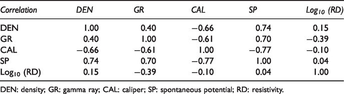
DEN: density; GR: gamma ray; CAL: caliper; SP: spontaneous potential; RD: resistivity.

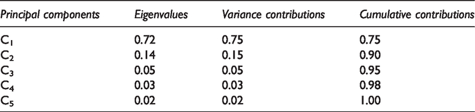
Firstly, we normalize the logs to the range of [−1, 1]. Secondly, we use the Jacobi method to calculate the PCs of input logs (Ren et al., 2018; Wang et al., 2017). For well A, we list the calculated eigenvalues, the variance contributions, and the cumulative contribution rate in Table 2. The variance contributions are very different from PCs to PCs. For the first PC, the variance contribution is 0.75 (accounting for 75% variation); for the last PC, the variance contribution is 0.02 (accounting for 2% variation). The cumulative variance contribution of the first three PCs is 95%, which is larger than 0.85. Therefore, the first three PCs can represent the most information variations of input logs. Finally, we use the first three PCs to fit an empirical function to reconstruct CNL and AC log. Since the standardized logs of GR, DEN, and log₁₀ (RD) contribute significantly to the PCs, we cross-plot them (Figure 6(a)) and compare them with the cross-plot of the first three PCs (Figure 6(b)), respectively. The cross-plot of GR, DEN, and log₁₀ (RD) logs is poorly separated, but the cross-plot of the first three PCs is well separated. After the PCA, the PCs are linearly independent.

Table 2.

The characteristics of eigenvalues and PCs.

Principal components	Eigenvalues	Variance contributions	Cumulative contributions
C₁	0.72	0.75	0.75
C₂	0.14	0.15	0.90
C₃	0.05	0.05	0.95
C₄	0.03	0.03	0.98
C₅	0.02	0.02	1.00

Figure 6.

The cross plots of the normalized logs (a) and the PCs (b). DEN: density.

Since all logs from different boreholes are de-noised, standardized, and normalized before PCA, the characteristics of eigenvalues and PCs of all wells in the study area are expected to be similar. We use the calculated PCs to perform regression and reconstruct CNL and AC log.

Results and discussions

CNL reconstruction

The lack of CNLs makes CBM interpretation and evaluation difficult. In this case, we use the proposed PCR model to regress a local reconstruction function shown as follows $\bar{C} = 25.75 - 3.18 C_{1} - 19.27 C_{2} - 1.30 C_{3}$ (6)where $\bar{C}$ is the reconstructed CNL, C₁ is the first PC, C₂ is the second PC, and C₃ is the third PC.

To monitor the reconstruction quality, we plot the logs of well A in Figure 7 and cross-plot the measured and reconstructed CNLs in Figure 8. In Figure 7, the formation between 560 m and 568 m is the No. 3 coal, where the DEN, GR, and SP logs have low responses, but the log₁₀ (RD), CAL, and CNL have high responses. The measured and reconstructed CNLs are generally similar in trend, mean, and scale. In Figure 8, the reconstructed and measured CNLs are almost linearly correlated, and the correlation coefficient is high (∼0.82). These are direct demonstrations of high reconstruction quality. Therefore, the proposed reconstruction method for the CNL is good enough for well A. Because all logs of other boreholes are standardized to well A, we use the same reconstruction function of well A to reconstruct the CNLs for all boreholes.

Figure 7.

The measured (solid curves) and the reconstructed (dash curve) logs of well A. DEN: density; GR: gamma ray; CAL: caliper; SP: spontaneous potential; RD: resistivity.

Figure 8.

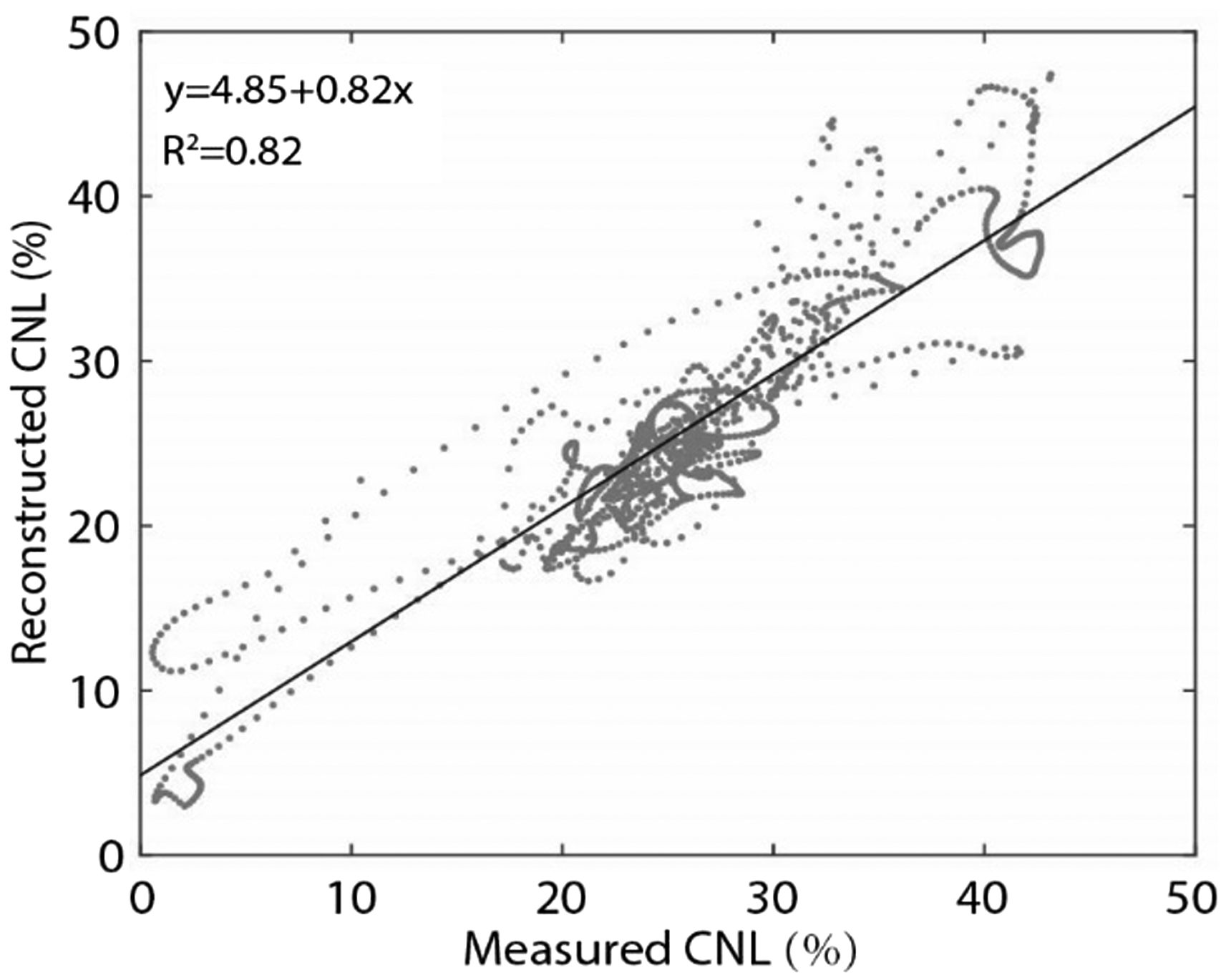
The cross plot of measured and reconstructed CNLs. CNL: compensated neutron log.

For the dry CBM reservoir, the CBM content is proportional to the CNL response and the coalbed thickness. Therefore, we define a relative gas content V_g, as shown in equation (7), to express the containing CBM content in the coalbed. $V_{g} = β Δ h \sum_{i = 1}^{N} {\bar{C}}_{i}$ (7)where the ${\bar{C}}_{i}$ is the reconstructed CNL response; Δh is the sample interval of logs, m; N is the sample numbers of logs within the coalbed; β is the calibration coefficient.

Well A has the complete logging suite and the actual measured CBM content (19.2 m³/t). We compute the gas content of the study area with equation (7). Firstly, we calculate the calibration coefficient β (13.3) through normalizing the sum of CNL response to the measured CBM content of well A. Secondly, we use equation (7) to calculate the gas content for other boreholes. Finally, we interpolate the gas content distribution of No. 3 coal in the study area, as shown in Figure 9(a).

Figure 9.

The distributions of estimated gas-content (a) and daily CBM production (b) of No. 3 coal in the study area.

In general, the gas content in the study area is relatively high (15.5–22.5 m³/t), but the distribution is not uniform. The top-middle and bottom-middle locations have the highest gas content; the top-right and middle-right locations have the lowest gas content; other locations have moderate gas content. Comparing Figure 9(a) with Figure 2, we find that the locations with a high gas content are located in the synclines, and this feature follows the regional characteristics of CBM enrichment (Peng et al., 2017; Teng et al., 2015; Zhang et al., 2013). Comparing Figure 9(a) with Figure 9(b), we find these two maps are similar. The top-left corner and the middle area have the highest values; the middle-right area has the lowest values; the transition between the high-value and the low-value areas is fast. These are additional demonstrations of the high reconstruction quality, although the influence factors of CBM production are complicated (Chen et al., 2019; Huang et al., 2019; Li and Wu, 2016; Song et al., 2005).

In summary, the proposed PCR model for the reconstruction of the CNL is relatively reliable and applicable in the study area.

AC log reconstruction

Similar to the CNL, the AC log is a crucial input for porosity evaluation and pore pressure prediction (Mavko et al., 2009; Zhang, 2011, 2013). Beside well A, other boreholes in the study area do not have AC logs. We use the measured AC log and the calculated PCs from well A to the AC log with multivariate regression. The local reconstruction function is shown as follows $\bar{A} = 263.64 - 43.10 C_{1} - 100.13 C_{2} - 8.91 C_{3}$ (8)where $\bar{A}$ is the reconstructed AC log, C₁ is the first PC, C₂ is the second PC, and C₃ is the third PC.

We plot the logs of well A in Figure 7 and cross-plot the measured and reconstructed AC logs in Figure 10. In Figure 7, the measured and reconstructed AC logs are generally similar in trend, mean, and scale. In the target coalbed (No. 3 coal), the measured and the reconstructed AC logs are almost identical. In Figure 10, the reconstructed and measured AC logs are linearly correlated, and the correlation coefficient is high (0.91). Therefore, the proposed reconstruction method for the AC log is good enough for well A.

Figure 10.

The cross plot of measured and reconstructed AC logs. AC: acoustic.

Conclusions

The main conclusions of this research include the following:

We have proposed a PCR model incorporating an MWA, a histogram calibration, a PCA, and a multivariate regression to reconstruct critical wireline logs for CBM evaluation. The model does not need core-related correlation, and there is no local optimization.

The PCR model can reliably reconstruct neutron and sonic logs, respectively. For well A, the reconstructed neutron and sonic logs are like the measured logs in trend, mean, and scale; the correlation coefficients between reconstructed and measured logs are high.

The predicted CBM-content distribution of the study area with the reconstructed neutron logs is not only following the regional distribution characteristics of CBM enrichment zones but also validated by the CBM production data.

Footnotes

Declaration of conflicting interests

The author(s) declared no potential conflicts of interest with respect to the research,authorship,and/or publication of this article.

Funding

The author(s) disclosed receipt of the following financial support for the research,authorship and/or publication of this article: This research was funded by the National Natural Science Foundation of China,grant numbers 41774128 and 41704115,the National Key R&D Program of China,grant number 2018YFB0605601,and a project funded by the Priority Academic Program Development of Jiangsu Higher Education Institutions.

ORCID iD

Tongjun Chen

References

Barrash

Morin

(1997) Recognition of units in coarse, unconsolidated braided-stream deposits from geophysical log data with principal components analysis. Geology 25: 687–690.

Chen

Wang

, et al. (2018) Deformation degree estimate for coal seam using well logs as input: A case study. Journal of Environmental and Engineering Geophysics 23: 89–101.

Chen

Cheng

, et al. (2019) Experimental study of the influences of water injections on CBM exploitation. Energy Sources Part A-Recovery Utilization and Environmental Effects 42: 1–12.

Faust

(1953) A velocity function including lithologic variation. Geophysics 18: 271–288.

Gardner

GHF

Gardner

Gregory

(1974) Formation velocity and density—The diagnostic basics for stratigraphic traps. Geophysics 39: 770–780.

Goutorbe

Lucazeau

Bonneville

(2006) Using neural networks to predict thermal conductivity from geophysical well logs. Geophysical Journal International 166: 115–125.

Hatherly

Medhurst

Zhou

(2016) Geotechnical evaluation of coal deposits based on the Geophysical Strata Rating. International Journal of Coal Geology 163: 72–86.

Honorio

BCZ

Drummond

Vidal

, et al. (2012) Well log denoising and geological enhancement based on discrete wavelet transform and hybrid thresholding. Energy Exploration & Exploitation 30: 417–433.

Huang

Liu

Cai

, et al. (2019) In situ stress distribution and its impact on CBM reservoir properties in the Zhengzhuang area, southern Qinshui Basin, North China. Journal of Natural Gas Science and Engineering 61: 83–96.

10.

Kang

Jiang

, et al. (2018) Environmental corrections of a dual-induction logging while drilling tool in vertical wells. Journal of Applied Geophysics 151: 309–317.

11.

Koizumi

(2007) Neutron capture logging calibration and data analysis for environmental contaminant assessment. Journal of Applied Geophysics 61: 111–131.

12.

(2016) Influence of pressure, coal structure and permeability on CBM well productivity at various burial depths in South Yanchuan Block, China. Earth Sciences Research Journal 20: D1–D9.

13.

Lorenzen

(2018) Multivariate linear regression of sonic logs on petrophysical logs for detailed reservoir characterization in producing fields. Interpretation 6: T543–T553.

14.

Mavko

Mukerji

Dvorkin

(2009) The Rock Physics Handbook. Cambridge: Cambridge University Press.

15.

Niebuhr

Wiese

Wilmsen

(2001) The cored Konrad 101 borehole (Cenomanian-Lower Coniacian, Lower Saxony): Calibration of surface and subsurface log data for the lower Upper Cretaceous of northern Germany. Cretaceous Research 22: 643–674.

16.

Peng

Zou

Zhou

, et al. (2017) Factors affecting coalbed methane (CBM) well productivity in the Shizhuangnan block of southern Qinshui basin, North China: Investigation by geophysical log, experiment and production data. Fuel 191: 427–441.

17.

Quartero

Bechtel

Leier

, et al. (2014) Gamma-ray normalization of shallow well-log data with applications to the Paleocene Paskapoo Formation, Alberta. Canadian Journal of Earth Sciences 51: 452–465.

18.

Ren

Zhang

Cui

, et al. (2016) A novel work flow of density-log normalization for coalbed-methane wells: An example from the Surat Basin in Australia. SPE Reservoir Evaluation & Engineering 19: 205–213.

19.

Ren

Tang

, et al. (2018) The identification of coal texture in different rank coal reservoirs by using geophysical logging data in northwest Guizhou, China: Investigation by principal component analysis. Fuel 230: 258–265.

20.

Rezaee

Kadkhodaie-Ilkhchi

Alizadeh

(2008) Intelligent approaches for the synthesis of petrophysical logs. Journal of Geophysics and Engineering 5: 12–26.

21.

Rolon

Mohaghegh

Ameri

, et al. (2009) Using artificial neural networks to generate synthetic well logs. Journal of Natural Gas Science and Engineering 1: 118–133.

22.

Rumelhart

McClelland

(1986) Parallel Distributed Processing: Explorations in the Microstructure of Cognition. Vol. 1. London: MIT Press.

23.

Scheevel

Payrazyan

(2001) Principal component analysis applied to 3D seismic data for reservoir property estimation. SPE Reservoir Evaluation & Engineering 4: 64–72.

24.

Siregar

Niu

Mostaghimi

, et al. (2017) Coal ash content estimation using fuzzy curves and ensemble neural networks for well log analysis. International Journal of Coal Geology 181: 11–22.

25.

Song

Zhao

Liu

, et al. (2005) The influence of tectonic evolution on the accumulation and enrichment of coalbed methane (CBM). Chinese Science Bulletin 50: 1–6.

26.

Teng

Yao

Liu

, et al. (2015) Evaluation of coal texture distributions in the southern Qinshui basin, North China: Investigation by a multiple geophysical logging method. International Journal of Coal Geology 140: 9–22.

27.

Wang

Chen

, et al. (2017) Quantitative thickness prediction of tectonically deformed coal using extreme learning machine and principal component analysis: A case study. Computers & Geosciences 101: 38–47.

28.

Guo

Yuan

, et al. (2010) Wavelet denoising of well logs and its geological performance. Energy Exploration & Exploitation 28: 87–95.

29.

Zhang

Liu

Yao

, et al. (2013) The control of structure on coalbed methane (CBM) enrichment in Zhengzhuang block of Qinshui Basin, China. Applied Mechanics and Materials 295–298: 3346–3349.

30.

Zhang

(2011) Pore pressure prediction from well logs: Methods, modifications, and new approaches. Earth-Science Reviews 108: 50–63.

31.

Zhang

(2013) Effective stress, porosity, velocity and abnormal pore pressure prediction accounting for compaction disequilibrium and unloading. Marine and Petroleum Geology 45: 2–11.

32.

Zhou

Esterle

(2008) Toward improved coal density estimation from geophysical logs. Exploration Geophysics 39: 124–132.

33.

Zhou

O’Brien

(2016) Improving coal quality estimation through multiple geophysical log analysis. International Journal of Coal Geology 167: 75–92.