Accelerated longitudinal designs: An overview of modelling,power,costs and handling missing data

Abstract

Longitudinal studies are often used to investigate age-related developmental change. Whereas a single cohort design takes a group of individuals at the same initial age and follows them over time, an accelerated longitudinal design takes multiple single cohorts, each one starting at a different age. The main advantage of an accelerated longitudinal design is its ability to span the age range of interest in a shorter period of time than would be possible with a single cohort longitudinal design. This paper considers design issues for accelerated longitudinal studies. A linear mixed effect model is considered to describe the responses over age with random effects for intercept and slope parameters. Random and fixed cohort effects are used to cope with the potential bias accelerated longitudinal designs have due to multiple cohorts. The impact of other factors such as costs and the impact of dropouts on the power of testing or the precision of estimating parameters are examined. As duration-related costs increase relative to recruitment costs the best designs shift towards shorter duration and eventually cross-sectional design being best. For designs with the same duration but differing interval between measurements, we found there was a cutoff point for measurement costs relative to recruitment costs relating to frequency of measurements. Under our model of 30% dropout there was a maximum power loss of 7%.

1 Introduction

Longitudinal studies are ideal for investigating age-related developmental change. When age is the time metric, different types of longitudinal designs can be distinguished according to the distribution of ages at recruitment. In a single cohort design all participants start out at the same age, whereas a study that recruits all available individuals with initial age in a specified range can be regarded as an ‘unstructured multicohort longitudinal design’. ¹ An accelerated longitudinal design (ALD) is a more structured multiple cohort design that takes multiple single cohorts, each one starting at a different age.

Figure 1 represents an ALD covering ages 0–7 with three cohorts, four annual measurements per subject and an overlap of two measurements between cohorts. Collection of measurements for this design would take 3 years (ignoring recruitment lags), compared to 7 years for a single cohort longitudinal study covering the same age range. This illustrates the main advantage of an ALD: its ability to span the age range of interest in a shorter period of time than would be possible with a single cohort longitudinal design. An additional advantage of a shorter study is that it should be less affected by dropout (where a participant leaves the study prematurely, so that no further measurements are possible). The trade-off for this shorter duration is the inherent missing data: by design, each subject’s measurement schedule covers only part of the age range of interest. This can be a problem when there is an age cohort effect, that is a systematic difference between people born at different times.

Figure 1.

A three cohort accelerated longitudinal design: recruitment ages are 0, 2 and 4 for cohort 1 (squares), cohort 2 (circles) and cohort 3 (triangles), respectively. Four annual measurements are taken, and there is an overlap of two measurements between successive cohorts: cohorts 1 and 2 both have measurements at ages 2 and 3, and cohorts 2 and 3 both have measurements at ages 4 and 5.

Design of an accelerated longitudinal study requires consideration of a number of parameters. Specific to this type of study are the number of cohorts and the extent of overlap between cohorts, whereas common to any longitudinal study, the frequency and timing of measurements also needs to be set. Varying these parameters may produce a large collection of candidate designs, so the question of how to choose the best design arises. In addition, the study may be constrained to a maximum duration, number of participants or number of measurements, and the relative costs of implementing different ALDs will play an important role in choosing between them.

Moerbeek ² considered the effect of number of cohorts, extent of overlap and frequency of measurement on power to detect a linear trend, for some specific ALDs. Tekle et al. ³ considered D-optimal designs for polynomial trends in age, for the case of non-overlapping cohorts. Fitzmaurice et al. ⁴ discussed cross-sectional and longitudinal effects and proposed a model for detecting differences between these effects, an approach that treats cohort effects as fixed. Miyazaki and Raudenbush ⁵ developed a test for cohort effects that also treats cohort as a fixed effect.

The aim of this paper is to provide a comprehensive discussion of the issues involved in the design and analysis of accelerated longitudinal studies. We provide a systematic investigation of characteristics of ALDs that affect power to detect a linear trend. We incorporate a model for study costs and identify the most cost-efficient designs. We also consider the impact of dropout and how to deal with cohort effects. Based on our results, we recommend some general guidelines for designing accelerated longitudinal studies.

2 Methods

2.1 Models and assumptions

2.1.1 Linear mixed model for responses

We adopt a polynomial linear mixed model for the responses $$y_{\mathrm{hi}}=X_{\mathrm{hi}}\beta +Z_{\mathrm{hi}}{b}_{\mathrm{hi}}+{\varepsilon }_{\mathrm{hi}}$$ (1) where y_hi is the vector of responses for subject i in cohort h, X_hi and Z_hi are design matrices for the fixed and random effects, β is the vector of fixed effects, and b_hi and ${\varepsilon }_{\mathrm{hi}}$ are vectors of subject-specific random effects and residual errors, respectively. The response data are hierarchical with three levels, longitudinal measurements are nested within a person and a person is nested within a cohort. We assume $b_{\mathrm{hi}}\sim N(0,D)$ , where D is the variance–covariance matrix of the random effects and let the (k, l) element of D be d_kl which is the covariance between the kth and lth random effects, ${\varepsilon }_{\mathrm{hi}}~N(0,{\Sigma }_{\mathrm{hi}})$ , and the residual errors from different individuals are assumed to be independent. In general Σ _hi can be used to account for additional correlation, such as serial correlation, over and above the correlation induced by the random effects, although it is often assumed that the residual errors are independent, that is ${\Sigma }_{\mathrm{hi}}=\sigma 2I$ . The residual errors and random effects are assumed to be mutually independent.

The form of the fixed effects design matrix X_hi will depend on the ages at which measurements are taken, the degree of the polynomial trend assumed for the responses and any other covariates (such as gender) that are included in the model. The form of the random effects design matrix Z_hi will depend on the random effects included in b_hi.

The covariance matrix for the responses from subject i in cohort h is $\text{var}(y_{\mathrm{hi}})=V_{\mathrm{hi}}=Z_{\mathrm{hi}}{\mathrm{DZ}}_{\mathrm{hi}}^T+{\Sigma }_{\mathrm{hi}}$ and the covariance matrix for the fixed effects estimates is $$\text{var}(\stackrel{\wedge }{\beta })=(\sum _{h=1}^N\sum _{i=1}^{n_h}{X}_{\mathrm{hi}}^T{V}_{\mathrm{hi}}^{-1}{X}_{\mathrm{hi}})-1$$ where n_h is the number of subjects in cohort h and N is the number of cohorts.

If only cohort-specific covariates such as age are included in the model, and measurements are taken at a common set of ages for individuals from the same cohort, then we can drop the i subscript on the design matrices and Σ to obtain $V_h=Z_h{\mathrm{DZ}}_h^T+{\Sigma }_h$ and $$\text{var}(\stackrel{\wedge }{\beta })=(\sum _{h=1}^N{n}_h{X}_h^T{V}_h^{-1}{X}_h)-1=[\sum _{h=1}^N{n}_h((X_h^T{\Sigma }_h^{-1}{X}_h)-1+D)-1]-1$$ The second expression for $\text{var}(\stackrel{\wedge }{\beta })$ above shows that for a single cohort longitudinal design (N = 1) with n subjects and no missing data $$\text{var}(\stackrel{\wedge }{\beta })=\frac{1}{n}((XT\Sigma -1X)-1+D)$$ Hence in this special case, dependence of $\text{var}({\stackrel{\wedge }{\beta }}_k)$ on D is only via d_kk, the variance of the kth random effects. However, this result does not hold for an ALD: where there are multiple cohorts starting at different ages then in general $\text{var}({\stackrel{\wedge }{\beta }}_k)$ does depend on the other elements of D and not just d_kk.

2.1.2 Linear trend with age

The model for a linear trend with age, and random effects for both the intercept and slope, is $$y_{\mathrm{hij}}={\beta }_0+{\beta }_1{a}_{\mathrm{hj}}+b_{0\mathrm{hi}}+b_{1\mathrm{hi}}{a}_{\mathrm{hj}}+{\epsilon }_{\mathrm{hij}}$$ (2) where a_hj is the age at which the jth measurement is taken for cohort h, and y_hij is the response at this age for subject i in cohort h. Hence $\beta =({\beta }_0,{\beta }_1)T,b_{\mathrm{hi}}=(b_{0\mathrm{hi}},b_{1\mathrm{hi}})T$ and $$X_h=Z_h=[1a_{h1}::1a_{{\mathrm{hm}}_h}]$$ where m_h is the number of measurements obtained for individuals in cohort h.

Where there is a linear trend, interest usually lies in estimation and inference regarding the slope parameter β₁, which represents the population average rate of change with age. The variance of the slope estimate ${\stackrel{\wedge }{\beta }}_1$ is the (2, 2) element of $\text{var}(\stackrel{\wedge }{\beta }),{\nu }_1=\text{var}({\stackrel{\wedge }{\beta }}_1)$ . For testing $H_0:{\beta }_1=0$ against $H_1:{\beta }_1={\beta }_1^{*}\ne 0$ at significance level α, the power is $$\Phi (\delta \sqrt{d_{22}}/\sqrt{{\nu }_1}-z_{1-\alpha /2})$$ (3) where $\delta ={\beta }_1^{*}/\sqrt{d_{22}}$ is the standardised effect size and Φ and z_x are the standard normal distribution function and x-quantile. For a given power, and assumptions regarding the relative size of each cohort (often assumed to be equal), this expression can be solved to give the required numbers of subjects in each cohort (easily implemented in R ⁶ ) using the function uniroot.

As described by Galbraith and Marschner, ⁷ for a single cohort longitudinal design with n subjects, m measurements per subject and uncorrelated residual errors ( $\Sigma =\sigma 2I$ ) $${\nu }_1=\frac{1}{n}(\frac{\sigma 2}{{\mathrm{ms}}_a^2}+d_{22})$$ where $s_a^2=(1/m)\sum _{j=1}^m(a_j-\overline{a})2$ is the sample variance of the measurement times. Here a_j is the jth measurement age and $\overline{a}$ is the mean of the measurement ages. For annual measurements this further simplifies to $${\nu }_1=\frac{1}{n}[\frac{12\sigma 2}{m(m-1)(m+1)}+d_{22}]$$ explicitly showing the lack of dependence on d₁₁ and d₁₂, and also on the initial measurement age.

2.1.3 Locally D-optimal designs

D-optimal designs are found by considering the determinant of the covariance matrix for the fixed effects estimates, $\text{det}(\text{var}(\stackrel{\wedge }{\beta }))$ , often referred to as the generalised variance. The optimal design is the one giving the smallest value for $\text{det}(\text{var}(\stackrel{\wedge }{\beta }))$ . Since D-optimal designs for linear mixed models depend on the unknown variance components, they are only locally optimal, as described by Ouwens et al., ⁸ for example.

2.1.4 Effect of centring age

As discussed by Fitzmaurice et al., ⁴ in a longitudinal study it is often desirable to centre the ages by subtracting some common age for all individuals in the study. This can avoid problems of collinearity when the model for the mean is a polynomial trend. For example, in an accelerated longitudinal study, the initial age a₁₁ of the youngest cohort might be subtracted from all ages so that $a_{\mathrm{hj}}-a_{11}$ is used in place of a_hj in the model.

From an analysis point of view, centring age is straightforward and does not require any further adjustments to the model. However, at the design stage of an accelerated longitudinal study, assumptions regarding the parameters of the assumed model will be required. In particular, assumptions regarding the elements of the random effects covariance matrix D will be needed, and some care needs to be taken to use the D matrix appropriate for the definition of ‘age’ to be used in calculating power and other criteria by which designs will be judged.

As an example, consider designing a study that adopts a linear model for the trend with age, and suppose D is obtained by fitting this model to data from a previous study where age was not centred. In this case d₁₁ represents between-subject variability in the response at age 0. If in designing the new study the formula for power (3) uses ages that have been centred by subtracting a₁₁, then the random effects covariance matrix to be used in that formula is $$D\text{'}=[d_{11}+2a_{11}{d}_{12}+a_{11}^2{d}_{22}{d}_{12}+a_{11}{d}_{22}{d}_{12}+a_{11}{d}_{22}{d}_{22}]$$ For a single cohort longitudinal design with no missing data this will not be an issue because then ν₁ only depends on the (2, 2) element of D which is d₂₂ for both D and $D\text{'}$ .

2.1.5 Model for costs

We assume that the costs of undertaking an accelerated longitudinal study can be split into the following four components: overheads, costs of recruiting subjects, costs of taking measurements, and ongoing costs related to the duration of the study. Hence $$\text{costs}=\text{overheads}+c_1\sum _{h=1}^N{n}_h+c_2\sum _{h=1}^N{n}_h{m}_h+c_{3}l$$ where c₁ is the cost of recruiting a subject, c₂ is the cost of taking a measurement, c₃ is the ongoing cost per year and l is the duration of the study. Assuming overheads contribute the same amount regardless of study design, the cost of different designs can be compared via the function $$C(c_1,c_2,c_3)=c_1\sum _{h=1}^N{n}_h+c_2\sum _{h=1}^N{n}_h{m}_h+c_{3}l$$ In particular, designs can be compared via total number of subjects by setting $c_2=c_3=0$ , via total number of measurements by setting $c_1=c_3=0$ and via duration by setting $c_1=c_2=0$ .

Expressing measurement and duration-related costs as multiples of the cost of recruiting a subject allows us to compare designs according to $$C(1,r_2,r_3)=\sum _{h=1}^N{n}_h+r_2\sum _{h=1}^N{n}_h{m}_h+r_{3}l$$ (4) where $r_2=c_2/c_1$ and $r_3=c_3/c_1$ , for $c_1\ne 0$ .

2.1.6 Cohort effects

By ‘cohort effect’ in this paper, we mean a birth or age cohort effect, that is a systematic difference between people born at different times. Discussing time trends in adult disease rates, Kuh and Ben-Shlomo ⁹ (chap. 9) describe ‘the major identifiable cohort effect, the effect of cigarette smoking on respiratory mortality’. This effect is obvious when age- and gender-specific lung cancer rates in the UK, for example, are plotted against year of birth. For males, the dramatic increase in rates starts for men born in the mid-1800s and peaks for those born at the turn of the century, reflecting the increase in smoking and its widespread adoption by servicemen in World War I. Of course, this particular effect is known to be caused by changes in (tar content adjusted) cigarette consumption, so that ‘birth cohort’ is really a proxy for this exposure. In other cases the reasons for the existence of a cohort effect may not be fully known.

When cohort effects exist, estimates of age-related change obtained from longitudinal and cross-sectional studies will differ. This is because a cross-sectional study samples people of different ages at a fixed time, so that age-related change is estimated from a mixture of different cohorts. For example, a cross-sectional study of respiratory function could be affected by the changes in smoking habits referred to above: the older people in the study may tend to have worse lung function not just because they are older, but also because of their smoking habits. In this case the cross-sectional estimate of change in lung function would indicate a steeper decline than the estimate obtained from a longitudinal study. Ware et al. ¹⁰ analyse a study of pulmonary function in never-smoking adults which finds evidence for a cohort effect not related to smoking.

Cohort effects can also have an impact on accelerated longitudinal studies. An ALD ‘pieces together’ trajectories from different cohorts, which may not be a valid representation of the whole age range when there are cohort effects. Since a single cohort longitudinal study consists of only one age cohort, it will produce an unbiased estimate of within-subject change for that cohort. However, the fact that there is only one cohort also makes it impossible to identify cohort effects from a single cohort longitudinal study. Cohort effects can be identified from accelerated longitudinal studies because they comprise multiple cohorts.

Some methods for modelling cohort effects in an ALD will be considered in this section. Section 2.1.7 considers methods that treat cohort effects as fixed, whereas Section 2.1.8 discusses a model with random cohort effects.

2.1.7 Fixed cohort effects

The most general model incorporating fixed cohort effects allows a completely different trend for each cohort. This approach is discussed by Miyazaki and Raudenbush. ⁵ When there is a linear trend with age, it is equivalent to allowing a different fixed intercept and slope for each cohort, so that the mean trend is $$E(y_{\mathrm{hij}})=({\beta }_{01}+\sum _{k=2}^N{\beta }_{0k}{\delta }_{\mathrm{hk}})+({\beta }_{11}+\sum _{k=2}^N{\beta }_{1k}{\delta }_{\mathrm{hk}})a_{\mathrm{hj}}$$ (5) where ${\delta }_{\mathrm{hk}}=1$ if h = k and 0 otherwise. This model has 2N fixed effects parameters. The null hypothesis of no cohort effect is given by $H_0:{\beta }_{\mathrm{ik}}=0,i=0,1;k=2,\dots ,N$ .

A simpler model, discussed by Fitzmaurice et al., ⁴ adds terms involving initial age to the model. For example, the linear trend model would include a single extra term in $a_{h1}$ $$E(y_{\mathrm{hij}})={\beta }_0+{\beta }_1{a}_{h1}+{\beta }_2{a}_{\mathrm{hj}}$$ (6) whereas a model with quadratic trend would include two extra terms, in $a_{h1}$ and $a_{h1}^2$ . The linear trend model has three parameters, and is special case of the full interaction model (5), with constraints ${\beta }_{12}=\dots ={\beta }_{1N}=0$ and ${\beta }_{0h}={\beta }_{02}(a_{h1}-a_{11})/(a_{21}-a_{11}),h=3,\dots ,N$ .

A model intermediate between models (5) and (6) can be conceptualised by allowing the fixed effects parameters to vary linearly with initial age. For the linear trend model, the intercept and slope for cohort h become ${\beta }_{0h}={\beta }_{01}+{\alpha }_0{a}_{h1}$ and ${\beta }_{1h}={\beta }_{11}+{\alpha }_1{a}_{h1}$ , respectively, so that $$E(y_{\mathrm{hij}})={\beta }_{0h}+{\beta }_{1h}{a}_{\mathrm{hj}}={\beta }_{01}+{\alpha }_0{a}_{h1}+{\beta }_{11}{a}_{\mathrm{hj}}+{\alpha }_1{a}_{h1}{a}_{\mathrm{hj}}$$ (7) This four-parameter model can be recognised as model (6) with the addition of an interaction between $a_{h1}$ and a_hj. The model is a special case of model (6), and in turn is a special case of model (5), with constraints ${\beta }_{0h}={\beta }_{02}(a_{h1}-a_{11})/(a_{21}-a_{11})$ and ${\beta }_{1h}={\beta }_{12}(a_{h1}-a_{11})/(a_{21}-a_{11}),h=3,\dots ,N$ .

More general versions of model (7) can be obtained by allowing the fixed effects parameters to vary smoothly, but not necessarily linearly, with initial age. For example, if we assume a quadratic relationship such that ${\beta }_{0h}={\beta }_{01}+{\gamma }_{01}{a}_{h1}+{\gamma }_{02}{a}_{h1}^2$ and ${\beta }_{1h}={\beta }_{11}+{\gamma }_{11}{a}_{h1}+{\gamma }_{12}{a}_{h1}^2$ , then $$E(y_{\mathrm{hij}})={\beta }_{01}+{\gamma }_{01}{a}_{h1}+{\gamma }_{02}{a}_{h1}^2+{\beta }_{11}{a}_{\mathrm{hj}}+{\gamma }_{11}{a}_{h1}{a}_{\mathrm{hj}}+{\gamma }_{12}{a}_{h1}^2{a}_{\mathrm{hj}}$$ (8)

Implied longitudinal and cross-sectional models

For models (6), (7) and (8), it is possible to write down the implied longitudinal and cross-sectional models. We assume here that the spacing between measurement times is the same for all individuals in the study, and let $l_j=a_{\mathrm{hj}}-a_{h1}$ , which depends only on j, not h.

The longitudinal model for cohort h obtains information on change by varying j for a fixed h (within-cohort), whereas the cross-sectional model at time j obtains information on change by varying h for a fixed j (cross-cohort). Table 1 presents the implied trends for each model (for simplicity, we have reparameterised models (7) and (8) in terms of β_j).

Table 1.

Longitudinal and cross-sectional trends for models (6), (7) and (8).

Model	Longitudinal trend (L)	Cross-sectional trend (C)	L = C if:
(6)	$({\beta }_0+{\beta }_1{a}_{h1})+{\beta }_2{a}_{\mathrm{hj}}$	$({\beta }_0-{\beta }_1{l}_j)+({\beta }_1+{\beta }_2)a_{\mathrm{hj}}$	${\beta }_1=0$
(7)	$({\beta }_0+{\beta }_1{a}_{h1})+$	$({\beta }_0-{\beta }_1{l}_j)+({\beta }_1+{\beta }_2-{\beta }_3{l}_j)$	${\beta }_1={\beta }_3=0$
	$({\beta }_2+{\beta }_3{a}_{h1})a_{\mathrm{hj}}$	$a_{\mathrm{hj}}+{\beta }_3{a}_{\mathrm{hj}}^2$
(8)	$({\beta }_0+{\beta }_1{a}_{h1}+{\beta }_2{a}_{h1}^2)+$	$({\beta }_0-{\beta }_1{l}_j+{\beta }_2{l}_j^2)+$	${\beta }_1={\beta }_2=$
	$({\beta }_3+{\beta }_4{a}_{h1}+{\beta }_5{a}_{h1}^2)a_{\mathrm{hj}}$	$({\beta }_1+{\beta }_3-2{\beta }_2{l}_j-{\beta }_4{l}_j+{\beta }_5{l}_j^2)a_{\mathrm{hj}}$  +	${\beta }_4={\beta }_5=0$
		$({\beta }_2+{\beta }_4-2{\beta }_5{l}_j)a_{\mathrm{hj}}^2+{\beta }_5{a}_{\mathrm{hj}}^3$

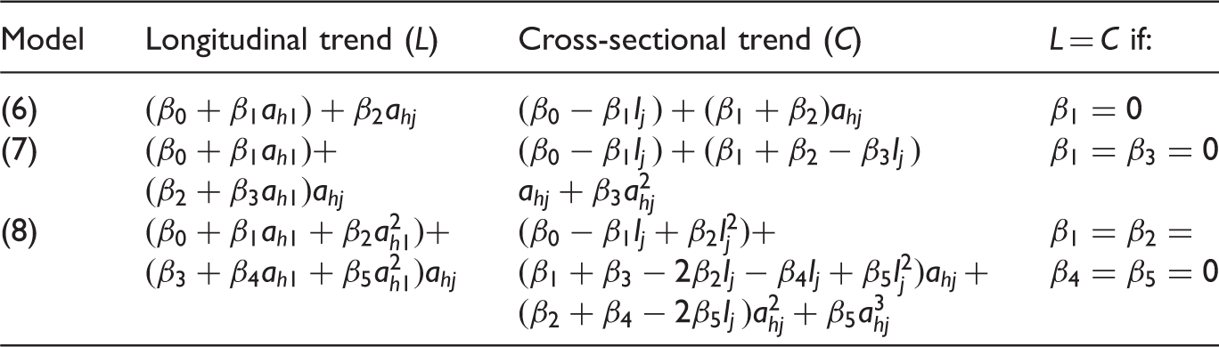
When the longitudinal and cross-sectional models coincide there is no cohort effect, and therefore the parameter constraints producing equality of these two models also define the null hypothesis of no cohort effect. The null hypothesis for each model is given in the final column of Table 1.

For model (6), the longitudinal model implies linear trends for the different cohorts that are parallel but shifted by the intercept term. This results in parallel linear trends at each time for the cross-sectional model. In model (7) the linear longitudinal trends are no longer parallel, leading to quadratic cross-sectional trends, whereas model (8) gives rise to cubic cross-sectional trends.

Comparison in region of overlap

If the curves for different cohorts are similar in regions of overlap, it may not be of concern that hypothesis tests indicate a significant difference in fixed effects parameters. This could be the case particularly when the regions of overlap are small, so that the information on the age range covered by a particular cohort comes largely from that cohort.

In this situation, fixed effects tests for differences between cohorts could be derived by integrating the absolute value of the difference between the estimated curves over the age range of overlap. Standard errors could be obtained via the delta method.

2.1.8 Random cohort effects

Another method of allowing for differences between cohorts would be to add a third level to the hierarchical model by including cohort-specific random effects. Under this approach, the model (1) becomes $$y_{\mathrm{hi}}=X_{\mathrm{hi}}\beta +W_h{\gamma }_h+Z_{\mathrm{hi}}{b}_{\mathrm{hi}}+{\varepsilon }_{\mathrm{hi}}$$ where the cohort-specific random effects ${\gamma }_h\hspace{1em}~N(0,G)$ . The covariance matrix for all measurements from cohort h has ith diagonal block $W_h{\mathrm{GW}}_h^T+Z_{\mathrm{hi}}{\mathrm{DZ}}_{\mathrm{hi}}^T+{\Sigma }_{\mathrm{hi}}$ and off-diagonal blocks $W_h{\mathrm{GW}}_h^T$ . Hence the cohort-specific random effects induce correlation between measurements for different people within the same cohort: people in the same cohort are ‘more alike’ than people from different cohorts.

2.1.9 Comparing designs when cohort effects are present

If cohort effects are anticipated at the design stage, two criteria of interest for comparing different designs might be:

Power to detect cohort effects; or

The determinant of the generalised variance corresponding to the vector of fixed effects.

Power to detect cohort effects

If cohort effects are modelled using model (6) then the null hypothesis of no cohort effect corresponds to equating a single parameter to zero: $H_0:{\beta }_1=0$ from Table 1. Hence the power to detect a cohort effect can be obtained from a similar formula to equation (3).

For model (7) the test for no cohort effect involves two parameters: $H_0:{\beta }_1={\beta }_3=0$ from Table 1, and for model (5) it involves $2N-2$ parameters. For these models we can use the approach described by Verbeke and Molenberghs ¹¹ (chap. 23) to calculate the power (or determine the required number of subjects for a given power). The approach is based on the fact that a test of $H_0:L\beta =0$ (where β is the vector of fixed effects and L is a matrix defining the null hypothesis contrast) can be based on the statistic $$F=(L\stackrel{\wedge }{\beta })T[L\stackrel{\wedge }{\text{var}}(\stackrel{\wedge }{\beta })LT]-1(L\stackrel{\wedge }{\beta })/\text{rank}(L)$$ which has an approximate F distribution with degrees of freedom equal to $\text{rank}(L)$ and $N-\text{rank}([X|Z])$ , under H₀. For a general value of $L\beta$ , Helms ¹² shows that the distribution of F can be approximated by a non-central F distribution, again with degrees of freedom $\text{rank}(L)$ and $N-\text{rank}([X|Z])$ , and with non-centrality parameter equal to $$(L\beta )T[L\text{var}(\stackrel{\wedge }{\beta })LT]-1(L\beta )$$ Hence the critical value corresponding to the chosen significance level can be determined from the distribution of F under the null, and this critical value used in calculating the power from the distribution of F under the alternative. Alternatively, for a fixed value of power, the required number of subjects can be obtained (for example using the function uniroot in R ⁶ ).

For the case of random cohort effects, testing the null hypothesis of no cohort effect corresponds to testing that some variance components are equal to zero. This is a test on the boundary of the parameter space, such that the null distribution is in general unknown. In this situation, power and sample size requirements could be obtained via simulation.

The determinant of the generalised variance corresponding to the vector of fixed effects

For comparing different designs (under the same model) with respect to how precisely the entire vector of fixed effects can be estimated, the D-optimality criterion described in Section 2.1.3 can be utilised. Note that the square root of the determinant of the generalised variance corresponding to the vector of fixed effects is proportional to the volume of the confidence ellipsoid of the joint distribution of the fixed effects.

2.1.10. Dropout

The relative impact of dropout on different ALDs depends on the dropout mechanism. Whilst this mechanism is in general unknown, it seems reasonable to assume that the overall level of dropout, as measured by the proportion w of subjects who have dropped out by the end of the study, will increase with study duration. Under this assumption, shorter duration designs will gain an advantage over longer duration designs.

In studying the impact of dropout on single cohort longitudinal designs, Galbraith and Marschner ⁷ adopted a Weibull model for the hazard of dropout: the rate at which individuals drop out at time t, conditional on remaining in the study up to time t, is $\lambda \gamma t\gamma -1$ . Under this model, the probability that a subject from cohort h will have exactly $j\le n_h$ measurements is $p_j=(1-w)t_j^{\gamma }-(1-w)t_{j+1}^{\gamma }$ . Given w, different patterns of dropout can be obtained by varying the single parameter γ: γ = 1 corresponds to a constant dropout rate over the course of the study, $\gamma <1$ implies dropout concentrated towards the start of the study and $\gamma >1$ implies dropout concentrated towards the end of the study.

The approach of Verbeke and Lesaffre ¹³ can then be used to simulate dropout patterns from a multinomial distribution with probabilities given by $p=(p_1,\dots ,p_{n_h})T$ . The conditional power for each simulated dropout pattern is then calculated, and we take the power for the design to be the mean of these conditional powers, as described fully in Galbraith and Marschner. ⁷ The approach assumes that the data missing due to dropout are missing at random. ¹⁴

In Section 4.2 we examine the pattern of dropout observed in a real study and investigate the impact of dropout for some ALDs.

3 Results

3.1 Identifying possible designs

With a completely general number and schedule of measurements for each cohort, the collection of candidate designs may be so large that it would be infeasible to investigate the properties of each one. Here we concentrate on ‘balanced’ ALDs, taken to mean ALDs with equally spaced measurements, the same number of measurements per subject, the same extent of overlap (number of common ages) between successive cohorts, and where the initial age for each cohort is an integer multiple of the interval between measurements. Under these conditions the measurement ages are $a_{\mathrm{hj}}=a_{11}+i[(h-1)(m-o)+j-1]/12$ , where m is the number of measurements per subject, i is the interval between measurements (in months) and o is the extent of overlap between cohorts. For a balanced ALD with N cohorts, the relationship $m=(A+(N-1)o)/N$ holds, where $A=12(a_{\mathrm{Nm}}-a_{11})/i+1$ is the number of ages to be covered by the study. Given A, the set of candidate designs is obtained by determining all possible combinations of N and o that yield integer values for m.

As an example of this approach, suppose we seek balanced ALDs to cover ages 11–18 with either a 6- or 12-month interval between measurements. Using the relationship given above yields 44 designs: 31 with a 6-month interval and 13 with a 12-month interval between measurements. Table 2 lists the 12-month interval designs.

Table 2.

ALDs covering ages 11–18 with a 12-month interval between measurements.

		Measurements	Number of
Design	Duration	per person	cohorts	Overlap
A	0	1	8	0
B	1	2	4	0
C	1	2	7	1
D	2	3	6	2
E	3	4	2	0
F	3	4	3	2
G	3	4	5	3
H	4	5	2	2
I	4	5	4	4
J	5	6	2	4
K	5	6	3	5
L	6	7	2	6
M	7	8	1	8 a

a

Overlap for single cohort design taken to be 8 since there is complete overlap between all subjects.

In the next section, the designs listed in Table 2 are used to illustrate how different ALDs can be compared.

3.2 Comparing designs

In this section we consider how to compare designs on the basis of power and the cost function (4) introduced in Section 2.1.5. Section 3.2.1 considers comparisons in the absence of dropout and cohort effects. In Section 3.2.2 the impact of dropout is considered, while Section 3.2.3 deals with cohort effects.

3.2.1 No dropout, no cohort effects

Power to detect a linear trend

We examined the effect of number of measurements per person, number of cohorts and extent of overlap on the power properties of the designs in Table 2.

Figure 2 plots the total number of subjects and total number of measurements required to achieve 90% power (3) to detect a linear trend in model (2) against the three attributes: measurements per person ( $m=\text{duration}+1$ ), number of cohorts (N) and extent of overlap (o), using design parameters D = I, $\sigma 2=1$ and $\delta =0.5$ . Designs are identified by letter. From these plots we see that both the total number of subjects and the total number of measurements display a monotonic relationship with m, but not with either N or o. Hence if (as in Moerbeek ² ) the objective is to limit either the total number of subjects or the total number of measurements, then the preferred design will be determined primarily by m. Specifically, if recruitment is difficult and only a limited number of subjects is available, then the design with the largest value of m (the single cohort longitudinal design) is best. On the other hand, if the aim is to minimise the total number of measurements, then the design with the smallest value of m (the cross-sectional design) is best.

Figure 2.

Total number of subjects (top) and total number of measurements (bottom) required to achieve 90% power to detect a linear trend, plotted as a function of number of measurements per person (left), number of cohorts (middle) and overlap (right), for the designs in Table 2 (identified by letter in the plot). Design parameters were D = I, $\sigma 2=1$ and $\delta =0.5$ .

Whilst m is the primary determinant for choosing between designs on these criteria, the value for N or o can be used to distinguish between designs with the same value for m. (For a fixed value of m, there is a monotonic relationship between N and o.) Multiple designs for the same value of m can be observed in Figure 2 for m = 2, 4, 5 and 6, and these designs are investigated further in Figure 3. It can be seen that for balanced ALDs with the same value for m (equivalently, the same duration), it is better to take fewer cohorts (equivalently, less overlap between cohorts), from the point of view of minimising either the total number of subjects or the total number of measurements. Figure 3 also shows that the effect is greater for shorter duration (smaller m) designs: whilst the increase in required number of subjects and measurements is noticeable for m = 2, the effect is barely perceptible for m = 6.

Figure 3.

Effect of number of cohorts/overlap on number of subjects/measurements for 90% power. The x-axis is number of cohorts for the left plots and overlap for the right plots, and the y-axis is total number of subjects for the top plots and total number of measurements for the bottom plots. Different coloured lines represent different durations (different m), and the points for the same duration/m are connected by lines.

Figure 4 gives an alternative presentation of the results, showing power as a function of the three determinants of cost: total number of subjects, total number of measurements and duration, for the designs in Table 2.

Figure 4.

Power to detect a linear trend, as a function of (a) total number of subjects; (b) total number of measurements; (c) duration for fixed total number of subjects (50); and (d) duration for fixed total number of measurements (112). Different curves/points represent different numbers of measurements per subject (m).

Figure 4(a) plots power as a function of total number of subjects. The power curves increase in height as m increases but there is a diminishing return with each additional measurement. Figure 4(b) plots power as a function of total number of measurements, showing a reverse ordering of the curves to Figure 4(a). These results are consistent with Figure 2, which shows horizontal cross-sections through Figure 4(a) and (b) at power 0.9. The effect of duration is shown in Figure 4(c) and (d). Since duration is fixed for a given design, we show the effect of duration for a fixed number of subjects (equal to 50) in Figure 4(c), and for a fixed number of measurements (equal to 112) in Figure 4(d) (corresponding to vertical slices in Figure 4(a) and (b), respectively).

We also examined the effect of the interval between measurements, by comparing the 12-month interval designs listed in Table 2 with the 6-month interval designs of the same duration. Figure 5 shows the total numbers of subjects and measurements required to achieve 90% power for the 44 designs, plotted against duration. It can be seen that the slightly smaller number of subjects often required for the 6-month interval designs is more than offset by the larger number of measurements taken for each subject, leading to a larger total number of measurements for all of the 6-month designs.

Figure 5.

Total numbers of subjects (left) and measurements (right) to achieve 90% power, for the designs in Table 2 and the corresponding 6-month interval designs, plotted against duration.

The results displayed in this section assume the design parameters D = I, $\sigma 2=1$ and $\delta =0.5$ . However, we also investigated the effect of varying the ratio of within to between-subject variability, $\sigma 2/d_{22}$ , from 1 (as assumed) to either 1/2 or 2, as well as the effect of varying the correlation between the random slope and intercept from 0 to either –0.8 or +0.8. Results (not shown) for these parameter values were qualitatively similar to those presented. In particular, the basis for choosing between designs in order to minimise either the total number of subjects or the total number of measurements would remain the same. Namely, for designs with the same interval between measurements:

If the aim is to minimise the total number of subjects, then designs with larger values for m are preferred, regardless of number of cohorts and overlap, although there is diminishing benefit as m continues to increase. For studies constrained to a maximum duration, this guideline would apply to the subset of candidate designs with duration less than the maximum (since larger m corresponds to longer duration).

If the aim is to minimise the total number of measurements, then designs with smaller values for m are preferred, regardless of number of cohorts and overlap.

For two designs with the same value of m (duration), the design with fewer cohorts (less overlap) is preferred, where the objective is to minimise either the total number of subjects or the total number of measurements.

In addition, decreasing the interval between measurements while keeping duration fixed (and hence increasing the number of measurements per person) led to an increase in the total number of measurements. The effect on total number of subjects appears to be small but could be in either direction.

It should be noted that these conclusions apply to choosing amongst balanced ALDs and rely on the assumptions of a linear trend and no cohort effects. In reality, other considerations may come into play when choosing a design, such as the need to check for linearity or for cohort effects, and the need to estimate variance components.

Costs

To illustrate how costs vary with design parameters, we use the total numbers of subjects and the resulting total number of measurements required to achieve 90% power for each design in Table 2. These are shown in the leftmost plots of Figure 2, for D = I, $\sigma 2=1$ and $\delta =0.5$ . The cost of each design is then calculated using equation (4).

We considered a grid of 36 values for (r₂, r₃) by cross-tabulating on the set of values $S=\{0.05,0.1,0.2,1,5,10\}$ . Figure 6 shows results for a subset of these values: $r_2\in \{0.05,0.1,0.2,1\}$ and $r_3\in \{0.2,1,5,10\}$ .

Figure 6.

Costs required to achieve 90% power, for the designs in Table 1, with $\sigma 2/d_{22}=1$ . The numbers at the top of each plot correspond to r₂, r₃. The minimum cost design is coloured red and the maximum cost design is coloured blue.

It can be seen that for a fixed value of r₃ (fixed column of plots), as r₂ increases, the minimum cost design shifts towards a smaller value for m. In other words, as the cost of taking a measurement increases relative to the cost of recruiting a subject, it becomes increasingly advantageous to take fewer measurements, and eventually once r₂ exceeds a certain value (depending on r₃), the cross-sectional design with one measurement per subject will always be the best. Similarly, for a fixed value of r₂ (fixed row of plots), as r₃ increases, the minimum cost design also shifts towards a smaller value for m. Hence as duration-related costs increase relative to recruitment costs, the advantage of a shorter duration increases. Again, the cross-sectional design with one measurement per subject will eventually achieve minimum cost once r₃ exceeds a certain value. Values in S × S not shown in Figure 6 yielded results consistent with these trends.

We also considered the effect of varying the ratio of within to between-subject variability, $\sigma 2/d_{22}$ , which was 1 for Figure 6. Results (not shown) suggest that decreasing $\sigma 2/d_{22}$ shifts the minimum cost design towards a smaller value for m, whilst increasing $\sigma 2/d_{22}$ shifts the minimum cost design towards a larger value for m. When correlation was introduced between the random slope and intercept, results (not shown) suggest that negative correlation tends to shift the minimum cost design towards a smaller value for m, whereas positive correlation shifts the minimum cost design towards a larger value for m.

We examined the effect of the interval between measurements in two different ways. First, the 12-month interval designs listed in Table 2 were compared with the 6-month interval designs with the same duration. Costs for the 44 designs were calculated using the total numbers of subjects and measurements required to achieve 90% power shown in Figure 5. For the purpose of comparing costs, without loss of generality we can set $r_3=0$ , since we should compare designs with the same duration. Hence the cost function (4) becomes simply a linear function of r₂, for a fixed total number of subjects and measurements. Figure 7 shows these linear functions for the six designs with duration 3. It can be seen that for values of r₂ less than a cutoff of about 0.011, the minimum overlap 6-month design has lowest cost, whereas for values of r₂ beyond this cutoff the minimum overlap 12-month design has lowest cost. The same effect can be observed for designs with integer durations 2–7: there is a cutoff point for r₂ below which the minimum overlap 6-month design has lowest cost, and above which the minimum overlap 12-month design has lowest cost. This cutoff decreases as duration increases, from about 0.042 at duration 2 to about 0.001 at duration 7. For duration 0 and 1 designs, the lowest cost design is always the minimum overlap 12-month design, regardless of r₂.

Figure 7.

Costs to achieve 90% power, for 6- and 12-month interval designs with duration 3, as a function of r₂.

The second investigation compared four different designs to cover ages 0–2 years, all using two cohorts with an overlap of one measurement. The interval between measurements was either 12, 6, 4, or 3 months, corresponding to m = 2, 3, 4, or 5. All of these designs have duration equal to 1 year. Figure 8 shows that for r₂ less than about 0.05, the lowest cost design is the 3-month interval design, and for $r_2>0.05$ , the lowest cost design is the 12-month interval design.

Figure 8.

Costs to achieve 90% power, for two-cohort designs to cover ages 0–2 with an overlap of 1 and 3, 4, 6, or 12 months between measurements.

3.2.2 Dropout

Dropout in the Longitudinal Study of Australian Children (LSAC)

Growing Up in Australia: The LSAC ¹⁵ recruited over 10,000 Australian children in 2004 and is following them up with the aim of addressing research questions related to child development and well-being. LSAC is a two-cohort ALD: the B cohort aged 0–1 initially and the K cohort aged 4–5 initially. As an initial investigation of the Weibull dropout model described in Section 2.1.10, we examined the pattern of dropout observed in LSAC.

Figure 9 shows the actual proportions of each cohort remaining in the study, as a function of study time, compared to a Weibull model with $\gamma =0.5$ . This model appears to be a good fit for LSAC.

Figure 9.

Dropout pattern in LSAC, showing the proportion remaining in the study as a function of study time. The letters represent observed proportions for the two cohorts (B and K), and the solid line is the fitted Weibull model with $\gamma =0.5$ .

Extent of power loss for different ALDs

Using the approach described in Section 2.1.10, we examined the impact of dropout for the designs listed in Table 2. Figure 10 shows the ratio of the power under 30% dropout to the power under no dropout, for γ = 1 (uniform dropout) and $\gamma =0.5$ (dropout concentrated more towards the start of the study, as observed for LSAC). The power under dropout was estimated as the mean of 10,000 simulations.

Figure 10.

Extent of power loss for 30% dropout, for the designs in Table 2, identified by letter, for γ = 1 (designs connected by dashed grey line) and $\gamma =0.5$ (designs connected by dotted grey line).

Figure 10 shows how, under the assumed models, the extent of power loss increases with duration. Hence the single cohort longitudinal design, with the longest duration, suffers the most power loss. Figure 10 also shows that the power loss is greater when dropout is concentrated more towards the start of the study. For the single cohort longitudinal design it can be seen that when 30% of participants drop out over the course of the study, the power is about 4% lower than if there were no dropout when γ = 1, and about 7% lower when $\gamma =0.5$ . For the other designs, the loss of power is smaller.

3.2.3 Cohort effects

Power to detect cohort effects

In this section we compare the ability of 11 of the designs listed in Table 2 to detect a cohort effect, assuming either model (6) or (7) holds. Designs A (cross-sectional) and M (single cohort longitudinal) are excluded from the comparison since they cannot distinguish cross-sectional from longitudinal effects and are therefore unable to detect cohort effects.

Figure 11 shows the total number of subjects and total number of measurements required to achieve 90% power to detect a cohort effect under model (6) with ${\beta }_1=0.5$ , and model (7) with ${\beta }_1={\beta }_3=0.2$ , in each case assuming D = I and $\sigma 2=1$ , where β₁ and β₃ are as defined in Table 1 (the results do not depend on the value of β₀ or β₂). The designs are identified by letter along the horizontal axis, and designs with the same value for m are joined by lines. For this particular choice of parameters, it can be seen that design E, with m = 4, is optimal for model (6), when judged by either total number of subjects or total number of measurements. It is also optimal for model (7) when judged by total number of subjects, however design B is best when judged by total number of measurements. Design K stands out as being the worst design: this may be because with seven measurements per subject and an overlap of six measurements, it is ‘almost’ a single cohort design (which has no power to detect a cohort effect). Again we see that for designs with the same value for m, it is better to have fewer cohorts (less overlap).

Figure 11.

Total number of subjects (top) and total number of measurements (bottom) required to achieve 90% power to detect a cohort effect under model (6) (left) and (7) (right), for designs B–L in Table 2 (identified by letter on the horizontal axis). Different coloured lines represent different durations (different m), and the points for the same duration/m are connected by lines.

Overall precision with which the vector of fixed effects can be estimated

This section compares designs according to the D-optimality criterion described in Section 2.1.3.

Figure 12 shows the determinant of the fixed effects covariance matrix under model (2) (no cohort effects) and with fixed cohort effects under models (6) and (7), assuming D = I and $\sigma 2=1$ . The determinants for a fixed 120 subjects, and for a fixed 840 measurements, are shown in separate plots.

Figure 12.

Determinant of fixed effects covariance matrix under models (2), (6) and (7), assuming D = I and $\sigma 2=1$ , for the designs in Table 2 (identified by letter on the horizontal axis). The left plot shows the determinant for a fixed 120 subjects, and the right plot for a fixed 840 measurements. Different coloured lines represent different durations (different m), and the points for the same duration/m are connected by lines.

Comparing designs for a fixed 120 subjects shows that while the single cohort longitudinal design is best in the absence of cohort effects, designs with fewer measurements per person can be better when there are cohort effects. For the chosen design parameters, design H, with five measurements per subject, is optimal for model (6), and design E, with four measurements per subject, is optimal for model (7).

For a fixed 840 measurements, the design with the lowest possible number of measurements per person is best for models (2) and (7). For model (6), design E, with four measurements per person, is optimal, although design B, with two measurements per person, is almost as good.

Under the assumption of fixed cohort effects, we again see that for designs with the same value for m, it is better to have fewer cohorts (less overlap).

Figure 13 shows some results for the case where cohort effects are assumed to be random rather than fixed. The three sets of results show the determinant for the case of no cohort effects, assuming a random cohort intercept only, and assuming a random cohort intercept and slope. The determinants for a fixed 120 subjects, and for a fixed 840 measurements, are shown in separate plots. We assume D = I, $\sigma 2=1$ , and G = 0.05 or $G=0.05I$ (for the case of one or two cohort random effects, respectively).

Figure 13.

Determinant of fixed effects covariance matrix with no cohort effects, a cohort random intercept, and both random intercept and slope, assuming D = I, $\sigma 2=1$ and G = 0.05 or $G=0.05I$ , for the designs in Table 2 (identified by letter on the horizontal axis). The left plot shows the determinant for a fixed 120 subjects, and the right plot for a fixed 840 measurements. Different coloured lines represent different durations (different m), and the points for the same duration/m are connected by lines.

We see that when random cohort effects are present, the best design for a fixed number subjects need not be the single cohort longitudinal design: design K performs best under the assumption of a random cohort intercept only, and design I performs best when random cohort intercept and slope are both present.

For a fixed 840 measurements, the cross-sectional design is best when there are no cohort effects or just a random intercept, but design D is best with both random intercept and slope.

Unlike the no cohort effects case and the fixed cohort effects case, where there are designs with the same value for m, we now see that it is better to have more cohorts (greater overlap).

4 Discussion and conclusions

ALDs are an attractive alternative to a single cohort longitudinal design when it is important to limit the duration of a study. They can also be preferable to an unstructured longitudinal study, where all individuals with initial age in a specified range are recruited, since they can be designed more efficiently. However, design of an accelerated longitudinal study can be a more complex task because additional design features, such as the number of cohorts and extent of overlap, require consideration.

In this paper we have discussed the issues that need to be considered when designing an accelerated longitudinal study, starting with a description of the linear mixed model framework for age-related trends in general and a linear trend in particular. We have considered criteria against which designs can usefully be judged (including cost considerations), the issue of cohort effects and the impact of dropout. We have shown how to generate all possible designs from the practically useful class of ‘balanced’ ALDs, and used this approach to illustrate how the design issues we have identified can be explored, and optimal designs according to the criteria mentioned can be chosen. In particular, we have investigated the impact of varying design parameters on these criteria.

Whilst we have tried to provide a comprehensive summary of design issues for accelerated longitudinal studies, in this paper we have not attempted to consider all possible designs or all possible trends with age. The motivation for considering balanced ALDs was that these designs represent a practically useful class that would be routinely considered when contemplating such a study. We are currently considering more general designs, including the problem of finding designs that either minimise cost for fixed variance or minimise variance for fixed cost. Similarly, the linear trend assumption represents a simple model that is often adopted at the design stage and is a useful starting point for exploring the effect of varying design parameters. We have also obtained some results for quadratic models that are broadly consistent with the linear trend, and the approaches we have described could be adapted to more complex trends. In addition, we have not looked at an exhaustive range of parameters (for example for the variance components), but rather have sought to describe general methods that can be used for different parameters.

Despite these limitations, our results suggest some broad guidelines for designing accelerated longitudinal studies.

In the absence of cohort effects, and for a fixed power to detect a linear trend, we found that the number of measurements per subject, m, was the primary determinant for choosing between designs when the criterion was to minimise either the total number of subjects or the total number of measurements: larger m designs are preferred by the former criterion, whereas smaller m designs are preferred by the latter, for a fixed interval between measurements. A similar result is known for conventional longitudinal studies with subjects measured at common, equally spaced, times over a fixed study period. ⁷ Whilst in that situation the result seems intuitively clear, it is not immediately obvious that it would also hold for ALDs, where number of cohorts and extent of overlap also come into play. Of course, whilst the result holds for the designs considered in this paper, there may be exceptions amongst the designs and design parameter values we have not considered. It is also important to recognise that this result (as with all others presented here) relies on the assumed model being correct. In practice, for example, it might be unwise to take only two measurements per person if the possibility of a nonlinear trend with age cannot be ruled out.

For two designs with the same value for m, the design with fewer cohorts (less overlap) is preferred, where the objective is to minimise either the total number of subjects or the total number of measurements. Again, this result relies on the assumed model being correct: intuitively if there were a linear trend and no difference between cohorts, then re-measuring the same age range would be inefficient. This is somewhat similar to the result for a conventional longitudinal study with straight line trend, whereby the best design for estimating the slope concentrates measurements at the start and end of the study period.

Finally, increasing the frequency of measurement for a fixed duration appears to have little effect on the required number of subjects, but increases the required total number of measurements.

To compare designs with respect to cost, we have used a three-component cost model incorporating recruitment, measurement and duration-related costs. For a fixed power to detect a linear trend, assuming no cohort effects, we found that as measurement costs increase relative to recruitment costs, the best design shifts towards smaller values for m, eventually becoming the cross-sectional design. Similarly, as duration-related costs increase relative to recruitment costs, the best design shifts towards shorter duration, and eventually the cross-sectional design again becomes the best. For designs with the same duration but differing interval between measurements, we found there was a cutoff point for measurement costs relative to recruitment costs, below which the smallest interval (highest frequency of measurement) design was best and above which the largest interval (lowest frequency of measurement) design was best.

The model we adopted for dropout assumes that the proportion of subjects who drop out by the end of the study increases with study duration. Under this model, studies with shorter duration will perform better. For the designs and models we considered, the maximum power loss for 30% dropout was about 7%, suggesting an increase in target power by this amount would be sufficient to allow for that level of dropout.

We have also presented some results for comparing designs when cohort effects are present. These results suggest that when the aim is either to detect cohort effects or to achieve a desired level of precision for estimating the entire vector of fixed effects estimates, there may be an advantage in increasing the number of measurements per subject. For designs with the same value of m, whilst fewer cohorts and less overlap were again better for the case of fixed cohort effects, the reverse was true for random cohort effects.

Finally, it should be mentioned that whilst this paper has focussed on design, there are issues surrounding the analysis of accelerated longitudinal studies that also need to be considered. For example, convergence problems can be encountered when fitting hierarchical linear mixed models in general, usually when the number of higher level units is small. For ALDs, there may be designs for which the combination of m, number of subjects, number of cohorts and overlap makes model fitting difficult. Hence even when the best design has been chosen, it may be prudent to try fitting the models to some simulated data, for example. In addition, to check the form of the actual trend with age, a sufficiently large value for m will be required.