Two-dimensional sparse Bayesian learning compressive beamforming with planar microphone array for acoustic source identification

Abstract

Two-dimensional (2D) compressive beamforming (CB) with planar microphone array for acoustic source identification has attracted much attention due to its advantages of wide identification space, applicability to both coherent and incoherent acoustic sources, and clear imaging. It realizes acoustic source identification by establishing and solving the underdetermined equations between the sound pressure measured by the microphone array and the source strengths of the discretized grid points in the target area. Convex relaxation algorithms and greedy algorithms are often used to solve these underdetermined equations. CB based on convex relaxation requires the sensing matrix to satisfy the restricted isometry property and needs large calculating consumption, which is unsuitable for large-scale problems. CB based on greedy algorithms may achieve a locally optimal solution instead of the global optimum, and it is easily affected by the coherence of the sensing matrix columns, so its performance is sensitive to the grid spacing. To take into account both the robustness of acoustic source identification performance and high computational efficiency, we adapted sparse Bayesian learning (SBL) to solve the above underdetermined equations and proposed a 2D-SBL-CB in this paper. It first assumes the signal prior and noise prior to derive the posterior probability distribution of the source strength, and then adaptively estimates the hyperparameters of the sparse prior of source strength based on a type-II maximum likelihood, i.e., by maximizing the evidence, to achieve source identification. Both simulations and experiment show that the proposed 2D-SBL-CB is robust to grid spacing and has stable source identification performance. It also enjoys high computational efficiency, strong spatial resolution ability, and strong anti-noise interference, with optimal overall performance.

Introduction

Beamforming based on planar microphone array is a popular acoustic source identification technology suitable for medium- and long-distance measurement,^1–4 which has been widely used in automobiles, airplanes, high-speed railways, wind power generation, and other fields.^5–8 Recently, two-dimensional (2D) compressive beamforming (CB) based on compressive sensing theory^9,10 has attracted much attention due to its advantages of wide identification space, applicability to both coherent and incoherent acoustic sources, and clear imaging.^11–14 Two-dimensional CB first assumes that the direction of arrival (DOA) of the acoustic source falls on the grid points formed by the discretized target area, then establishes an underdetermined equation system between the sound pressure vector measured by the array microphones and the strength distribution of grid points, finally estimates the DOA and strength of the acoustic sources by solving this underdetermined equation system under the sparse constraint.

Convex relaxation algorithms^15–18 and greedy algorithms^19–21 are often used to solve these underdetermined equations. CB based on convex relaxation replaces the original minimum $l_0$ norm with the minimized $l_1$ norm as the sparse constraint based on the fact that the $l_0$ norm is approximately equivalent to the $l_1$ norm when the sensing matrix satisfies the restricted isometry property (RIP), ²² transforming the intractable non-convex constrained optimization problem into a convex constrained one that easy to solve. Solving this convex constrained optimization problem with some well-established convex optimization algorithms (such as the interior point method), the source strength distribution can be obtained, and then the acoustic source identification can be achieved. Benefiting from the property of convex function, CB based on convex relaxation can obtain the global optimum. However, it requires the sensing matrix to satisfy RIP and needs large computational consumption, which is unsuitable for large-scale problems. The iterative reweighted $l_1$ norm minimization (IRl1) is a typical convex relaxation method. CB based on greedy algorithms selects the basis vector (columns of the sensing matrix) that has the most coherence with the measured signal from the sensing matrix one by one and gradually constructs support set to achieve a sparse approximation of the microphone sound pressure signal to achieve source identification. Matching pursuit (MP), orthogonal matching pursuit (OMP), and generalized orthogonal matching pursuit (gOMP) are all typical greedy algorithms. CB based on greedy algorithms usually enjoys high computational efficiency, but they may obtain locally optimal solution instead of the global optimum. Besides, CB based on greedy algorithms is sensitive to the coherence of sensing matrix columns, and their performance is significantly affected by grid spacing.

In recent, the literatures^23–26 introduced sparse Bayesian learning (SBL) to solve the mathematical model of CB with linear microphone array. It utilizes the Bayesian inference to determine the posterior probability distribution of source strength according to the likelihood function and the prior model, and then adaptively learn the hyperparameters of source strength. One-dimensional CB based on SBL demonstrates high computational efficiency and good performance. However, the linear microphone array is suitable for one-dimensional source identification scenario where the acoustic source is co-planar with the microphone array. This means that the one-dimensional SBL-CB with linear microphone array can only identify the elevation of source, but not the azimuth. Therefore, its application scenario is limited. Compared with CB with linear microphone array, CB with planar microphone array can identify both the elevation and azimuth of source in the half space in front of the array, which leads to a wider range of application scenarios. However, its computational burden will increase significantly. In view of this, to achieve both good acoustic source identification performance and high computational efficiency, we developed the SBL-based solver for 2D CB and established 2D-SBL-CB with planar microphone array for acoustic source identification. It first assumes the signal prior and noise prior to derive the posterior probability distribution of the source strength and then adaptively estimates the hyperparameters of the sparse prior of source strength based on a type-II maximum likelihood, i.e., by maximizing the evidence, to achieve source identification.

Planar microphone array measurement model

Figure 1 illustrates the measurement model of a planar microphones array in the plane wave conduction sound field, in which the symbols “•” denote microphones. Define that the spherical coordinate origin is at the center of the array, and the xoy plane coincides with the array plane. Suppose there are $I$ sources. The DOA of the $i\text{th}$ source is $\left({\theta }_{{\mathrm{S}}_i},{\varphi }_{{\mathrm{S}}_i}\right)$ . ${\theta }_{{\mathrm{S}}_i}\in \left[0°,90°\right]$ is the elevation angle, corresponding to the angle between the DOA of the $i\text{th}$ source and the z-axis. ${\varphi }_{{\mathrm{S}}_i}\in [0°,360°)$ is the azimuth angle, corresponding to the angle between the projection of DOA of the $i\text{th}$ source on the xoy plane and the x-axis. Assemble the DOAs of all sources into a matrix ${\mathbf{\Omega }}_{\mathrm{S}}=\left[{\left[{\theta }_{\mathrm{S}1},{\varphi }_{\mathrm{S}1}\right]}^{\mathrm{T}},{\left[{\theta }_{\mathrm{S}2},{\varphi }_{\mathrm{S}2}\right]}^{\mathrm{T}},\cdot \cdot \cdot ,{\left[{\theta }_{\mathrm{S}I},{\varphi }_{\mathrm{S}I}\right]}^{\mathrm{T}}\right]$ , in which the superscript “ $\mathrm{T}$ ” denotes the transpose operator. Let $l=\mathrm{1,2},\cdot \cdot \cdot ,L$ denote the snapshot index. $s_{i,l}\in \mathbb{C}$ is the strength of the $i\text{th}$ source in the $l\text{th}$ snapshot, and ${\mathbf{s}}_i=\left[s_{i,1},s_{i,2},\cdot \cdot \cdot ,s_{i,L}\right]\in {\mathbb{C}}^{1\times L}$ is the strength vector of the $i\text{th}$ source in all the $L$ snapshots. The source strength is defined as the complex sound pressure at the Cartesian coordinate origin.

Figure 1.

Measurement model of a planar microphones array in the plane wave conduction sound field.

The sound pressure $\mathbf{P}\in {\mathbb{C}}^{Q\times L}$ of all the $Q$ microphones in all the $L$ snapshots can be expressed in the frequency domain as ² $\mathbf{P}=\mathbf{A}\left({\mathbf{\Omega }}_{\mathrm{S}}\right)\mathbf{S}$ (1)where $\mathbf{A}\left({\mathbf{\Omega }}_{\mathrm{S}}\right)\in {\mathbb{C}}^{Q\times I}$ is the transfer matrix, and $\mathbf{S}\in {\mathbb{C}}^{I\times L}$ is the strength matrix of all the $I$ sources in all the $L$ snapshots. $\mathbf{P}=\left[\begin{array}{ccc}{p}_{\mathrm{1,1}}& \cdot \cdot \cdot & p_{1,L}\\ ⋮& \ddots & ⋮\\ p_{Q,1}& \cdot \cdot \cdot & p_{Q,L}\end{array}\right]\in {\mathbb{C}}^{Q\times L}$ (2) $\mathbf{A}\left({\mathbf{\Omega }}_{\mathrm{S}}\right)=\left[\begin{array}{ccc}{\mathrm{e}}^{\mathrm{j}2\pi \left(\sin {\theta }_{\mathrm{S}1}\cos {\varphi }_{\mathrm{S}1}{x}_{\mathrm{M}1}+\sin {\theta }_{\mathrm{S}1}\sin {\varphi }_{\mathrm{S}1}{y}_{\mathrm{M}1}\right)/\lambda }& \dots & {\mathrm{e}}^{\mathrm{j}2\pi \left(\sin {\theta }_{\mathrm{S}I}\cos {\varphi }_{\mathrm{S}\mathrm{I}}{x}_{\mathrm{M}1}+\sin {\theta }_{\mathrm{S}I}\sin {\varphi }_{\mathrm{S}I}{y}_{\mathrm{M}1}\right)/\lambda }\\ ⋮& \ddots & ⋮\\ {\mathrm{e}}^{\mathrm{j}2\pi \left(\sin {\theta }_{\mathrm{S}1}\cos {\varphi }_{\mathrm{S}1}{x}_{\mathrm{M}Q}+\sin {\theta }_{\mathrm{S}1}\sin {\varphi }_{\mathrm{S}1}{y}_{\mathrm{M}Q}\right)/\lambda }& \cdots & {\mathrm{e}}^{\mathrm{j}2\pi \left(\sin {\theta }_{\mathrm{S}I}\cos {\varphi }_{\mathrm{S}I}{x}_{\mathrm{M}Q}+\sin {\theta }_{\mathrm{S}I}\sin {\varphi }_{\mathrm{S}I}{y}_{\mathrm{M}Q}\right)/\lambda }\end{array}\right]\in {\mathbb{C}}^{Q\times I}$ (3) $\mathbf{S}=\left[\begin{array}{ccc}{s}_{\mathrm{1,1}}& \dots & s_{1,L}\\ ⋮& \ddots & ⋮\\ s_{I,1}& \cdots & s_{I,L}\end{array}\right]\in {\mathbb{C}}^{I\times L}$ (4)With the noise interference, the ${\mathbf{P}}^{\star }\in {\mathbb{C}}^{Q\times L}$ measured by the microphones should include the theoretical sound pressure $\mathbf{P}$ and the noise interference $\mathbf{N}\in {\mathbb{C}}^{Q\times L}$ in measurement, that is, ${\mathbf{P}}^{\star }=\mathbf{P}+\mathbf{N}$ (5)

Signal-to-noise ratio (SNR) is defined as $\text{SNR}=20{\log }_{10}\left({\Vert \mathbf{P}\Vert }_{\mathrm{F}}/{\Vert \mathbf{N}\Vert }_{\mathrm{F}}\right)$ , where ${\Vert \cdot \Vert }_{\mathrm{F}}$ denotes the Frobenius norm of a matrix.

Compressive beamforming

Compressive beamforming discretizes the target area into $G$ grid points along the $\theta$ and $\varphi$ directions with certain intervals. DOA of the $g\text{th}$ grid point is denoted by $\left({\theta }_{\mathrm{G}g},{\varphi }_{\mathrm{G}g}\right)$ . Let ${\mathbf{\Omega }}_{\mathrm{G}}=\left[{\left[{\theta }_{\mathrm{G}1},{\varphi }_{\mathrm{G}1}\right]}^{\mathrm{T}},{\left[{\theta }_{\mathrm{G}2},{\varphi }_{\mathrm{G}2}\right]}^{\mathrm{T}},\cdot \cdot \cdot ,{\left[{\theta }_{\mathrm{G}G},{\varphi }_{\mathrm{G}G}\right]}^{\mathrm{T}}\right]\in {\mathbb{R}}^{2\times G}$ denotes the DOA matrix of all the $G$ grid points. Suppose that each grid point corresponds to the DOA of a potential acoustic source, and the acoustic source identification can be transformed as solving the following equations. ${\mathbf{P}}^{\star }=\mathbf{A}\left({\mathbf{\Omega }}_{\mathrm{G}}\right)\mathbf{S}+\mathbf{N}$ (6)where $\mathbf{A}\left({\mathbf{\Omega }}_{\mathrm{G}}\right)=\left[\mathbf{a}\left({\theta }_{\mathrm{G}1},{\varphi }_{\mathrm{G}1}\right),\mathbf{a}\left({\theta }_{\mathrm{G}2},{\varphi }_{\mathrm{G}2}\right),\cdot \cdot \cdot ,\mathbf{a}\left({\theta }_{\mathrm{G}G},{\varphi }_{\mathrm{G}G}\right)\right]\in {\mathbb{C}}^{Q\times G}$ is the sensing matrix, $\mathbf{S}={\left[{\mathbf{s}}_1^{\mathrm{T}},{\mathbf{s}}_2^{\mathrm{T}},\cdot \cdot \cdot ,{\mathbf{s}}_G^{\mathrm{T}}\right]}^{\mathrm{T}}$ $\in {\mathbb{C}}^{G\times L}$ is the unknown strength matrix of all grid points in all the $L$ snapshots, and ${\mathbf{s}}_g\in {\mathbb{C}}^{1\times L}$ is the source strength of the $g\text{th}$ grid point in all the $L$ snapshots.

Since the number of microphones is usually far less than that of grid points, that is, $Q\ll G$ , equation (6) is underdetermined and a typical ill-posed inverse problem. To solve this ill-posed inverse problem, based on the fact that the main acoustic sources are usually sparsely distributed in space, CB applies a sparse constraint on the source strength using the $l_{2,p}$ norm ( $0\le p\le 1$ , which is the $l_p$ norm in the case of a single snapshot model), and transforms the problem as the following $l_{2,p}$ norm ( $l_p$ norm) minimization problem. $\widehat{\mathbf{S}}=\underset{\mathbf{S}\in {\mathbb{C}}^{G\times L}}{\mathrm{a}\mathrm{r}\mathrm{g}\mathrm{m}\mathrm{i}\mathrm{n}}{\Vert \mathbf{S}\Vert }_{2,p}^p\hspace{0.17em}\mathrm{s}.\mathrm{t}.\hspace{0.17em}{\Vert {\mathbf{P}}^{\star }-\mathbf{A}\left({\mathbf{\Omega }}_{\mathrm{G}}\right)\mathbf{S}\Vert }_{\mathrm{F}}\le \epsilon$ (7)where, $\epsilon$ is the tolerance of noise $\mathbf{N}$ , and ${\Vert \mathbb{A}\Vert }_{2,p}$ is the $l_{2,p}$ norm. ${\Vert \mathbf{S}\Vert }_{2,p}^p$ is as follows. ${\Vert \mathbf{S}\Vert }_{2,p}^p=\{\begin{array}{l}{\displaystyle \sum }_{g=1}^G{\Vert {\mathbf{S}}_{g,:}\Vert }_2^p,\hspace{0.17em}\text{if}\hspace{0.17em}p\ne 0\\ \left|\left\{g|{\Vert {\mathbf{S}}_{g,:}\Vert }_2>0\right\}\right|=\left|\left\{g|{\mathbf{S}}_{g,:}\ne \mathbf{0}\right\}\right|,\hspace{0.17em}\text{if}\hspace{0.17em}p=0\end{array}$ (8)where, ‖▪‖₂ is the $l_2$ norm of a vector, and |▪| is the potential of a set. CB utilizes the sparse recovery algorithms to solve equation (7) to obtain the strength distribution of grid points S, so as to achieve the acoustic source identification.

Two-dimensional sparse Bayesian learning compressive beamforming

The 2D-SBL-CB uses a hierarchical two-level Bayesian inference to reconstruct sparse estimates from the sound pressure signal measured by the microphones. The first level assumes the signal prior and noise prior to derive the posterior probability distribution of the source strength. The second level adaptively estimates the hyperparameters of the sparse prior of source strength based on a type-II maximum likelihood, that is, by maximizing the evidence. The 2D-SBL-CB adaptively estimates the hyperparameters from the measured sound pressure signals to obtain a sparse and robust estimate of the source strength distribution.

Based on the model shown in equation (6), 2D-SBL-CB assumes that the source strength is the zero-mean complex Gaussian with a covariance matrix $\mathbf{\Gamma }=\text{Diag}\left({\mathbf{\sigma }}_{\mathrm{S}}\right)\in {\mathbb{C}}^{G\times G}$ . $\text{Diag}(\cdot )$ means constructed as a diagonal matrix with the elements in brackets as diagonal elements. ${\mathbf{\sigma }}_{\mathrm{S}}=\left[{\sigma }_{\mathrm{S}1},{\sigma }_{\mathrm{S}2},\cdots ,{\sigma }_{\mathrm{S}G}\right]$ controls the sparsity of the source strength distribution, and is the hyperparameters to be solved. ${\sigma }_{\mathrm{S}g}$ denotes the variance of the $g\text{th}$ element of ${\mathbf{S}}_{:,l}$ . For the multi-snapshot scenario, each column vector of $\mathbf{S}$ has the same sparse profile, and the model parameters are assumed to be independent under each snapshot. Therefore, the prior distribution of source strength can be written as $p\left(\mathbf{S}\right)=\stackrel{L}{\underset{l=1}{\mathrm{\Pi }}}\hspace{0.17em}p\left({\mathbf{S}}_{:,\hspace{0.17em}l}\right)=\stackrel{L}{\underset{l=1}{\mathrm{\Pi }}}\hspace{0.17em}\mathcal{CN}\left({\mathbf{S}}_{:,\hspace{0.17em}l}|\hspace{0.17em}\mathbf{0},\hspace{0.17em}\mathbf{\Gamma }\right)$ (9)where $\mathrm{\Pi }$ is the multiplication operator. Similarly, assuming that the noise is also zero-mean complex Gaussian, independent both across sensors and snapshots, the prior distribution of noise can be written as $p\left(\mathbf{N}\right)=\stackrel{L}{\underset{l=1}{\mathrm{\Pi }}}p\left({\mathbf{N}}_{:,\hspace{0.17em}l}\right)=\stackrel{L}{\underset{l=1}{\mathrm{\Pi }}}\mathcal{CN}\left({\mathbf{N}}_{:,l}|\hspace{0.17em}\mathbf{0},\hspace{0.17em}{\mathbf{\Sigma }}_{\mathrm{N}}\right)$ (10)where ${\mathbf{\Sigma }}_{\mathrm{N}}={\sigma }_{\mathrm{N}}^2\mathbf{I}\in {\mathbb{C}}^{Q\times Q}$ ( $\mathbf{I}\in {\mathbb{R}}^{Q\times Q}$ is the identity matrix) is the covariance matrix of the noise distribution. Therefore, the data likelihood is $p({\mathbf{P}}^{\star }|\mathbf{S})=\stackrel{L}{\underset{l=1}{\mathrm{\Pi }}}\hspace{0.17em}p({\mathbf{P}}_{:,l}^{\star }|{\mathbf{S}}_{:,l})=\stackrel{L}{\underset{l=1}{\mathrm{\Pi }}}\hspace{0.17em}\mathcal{CN}({\mathbf{P}}_{:,l}^{\star }|\hspace{0.17em}\mathbf{A}\left({\mathbf{\Omega }}_{\mathrm{G}}\right){\mathbf{S}}_{:,l},\hspace{0.17em}{\mathbf{\Sigma }}_{\mathrm{N}})$ (11)

Based on the Gaussian prior shown in equation (9) and the likelihood shown in equation (11), the posterior distribution of the source strength can be obtained as $p\left(\mathbf{S}|\hspace{0.17em}{\mathbf{P}}^{\star }\right)\propto p\left({\mathbf{P}}^{\star }|\hspace{0.17em}\mathbf{S}\right)p\left(\mathbf{S}\right)=\stackrel{L}{\underset{l=1}{\mathrm{\Pi }}}\hspace{0.17em}\mathcal{CN}\left({\mathbf{\mu }}_l,\hspace{0.17em}{\mathbf{\Sigma }}_{\mathrm{S}}\right)$ (12)where ${\mathbf{\mu }}_l\in {\mathbb{C}}^{G\times 1}$ and ${\mathbf{\Sigma }}_{\mathrm{S}}\in {\mathbb{C}}^{G\times G}$ are the mean and covariance of the posterior distribution of $\mathbf{S}$ , respectively. ${\mathbf{\mu }}_l=\mathbf{\Gamma }{\left(\mathbf{A}\left({\mathbf{\Omega }}_{\mathrm{G}}\right)\right)}^{\mathrm{H}}{\mathbf{\Sigma }}_{\mathrm{P}}^{-1}{\mathbf{P}}_{:,l}^{\star }$ (13) ${\mathbf{\Sigma }}_{\mathrm{S}}=\mathbf{\Gamma }-\mathbf{\Gamma }\mathbf{A}{\left({\mathbf{\Omega }}_{\mathrm{G}}\right)}^{\mathrm{H}}{\mathbf{\Sigma }}_{\mathrm{P}}^{-1}\mathbf{A}\left({\mathbf{\Omega }}_{\mathrm{G}}\right)\mathbf{\Gamma }$ (14)where ${\mathbf{\Sigma }}_{\mathrm{P}}\in {\mathbb{C}}^{Q\times Q}$ is the covariance matrix of measured sound pressure ${\mathbf{P}}^{\star }$ ${\mathbf{\Sigma }}_{\mathrm{P}}=\mathbb{E}\left({\mathbf{P}}_{:,l}^{\star }{({\mathbf{P}}_{:,l}^{\star })}^{\mathrm{H}}\right)={\sigma }_{\mathrm{N}}^2\mathbf{I}+\mathbf{A}\left({\mathbf{\Omega }}_{\mathrm{G}}\right)\mathbf{\Gamma }{\left(\mathbf{A}\left({\mathbf{\Omega }}_{\mathrm{G}}\right)\right)}^{\mathrm{H}}$ (15) $\mathbb{E}(\cdot )$ denotes the expectation operator. The 2D-SBL-CB uses the evidence to estimate hyperparameters ${\sigma }_{\mathrm{N}}^2$ and ${\mathbf{\sigma }}_{\mathrm{S}}$ . According to the total probability theorem, the distribution of the measured sound pressure vector (evidence) $p\left({\mathbf{P}}^{\star }\right)$ can be obtained as $p\left({\mathbf{P}}^{\star }\right)=\int p\left({\mathbf{P}}^{\star }|\mathbf{S}\right)p\left(\mathbf{S}\right)\mathrm{d}\mathbf{S}=\frac{{\mathrm{e}}^{-\text{tr}\left({\left({\mathbf{P}}^{\star }\right)}^{\mathrm{H}}{\mathbf{\Sigma }}_{\mathrm{P}}^{-1}{\mathbf{P}}^{\star }\right)}}{{\left({\pi }^Q\mathrm{d}\mathrm{e}\mathrm{t}\left({\mathbf{\Sigma }}_{\mathrm{P}}\right)\right)}^L}$ (16)where $\text{tr}(\cdot )$ and $\mathrm{d}\mathrm{e}\mathrm{t}(\cdot )$ denote the trace and determinant of the matrix, respectively. The hyperparameters ${\mathbf{\sigma }}_{\mathrm{S}}$ are estimated with a type-II maximum likelihood (i.e., maximizing the evidence) ${\widehat{\mathbf{\sigma }}}_{\mathrm{S}}=\mathrm{a}\mathrm{r}\mathrm{g}\underset{{\sigma }_{\mathrm{S}g}\ge 0}{\max }\hspace{0.17em}\left(\ln p\left({\mathbf{P}}^{\star }\right)\right)=\mathrm{a}\mathrm{r}\mathrm{g}\hspace{0.17em}\underset{{\sigma }_{\mathrm{S}g}\ge 0}{\max }\hspace{0.17em}\left(-\text{tr}\left({\left({\mathbf{P}}^{\star }\right)}^{\mathrm{H}}{\mathbf{\Sigma }}_{\mathrm{P}}^{-1}{\mathbf{P}}^{\star }\right)-L\hspace{0.17em}\ln \hspace{0.17em}\mathrm{d}\mathrm{e}\mathrm{t}\left({\mathbf{\Sigma }}_{\mathrm{P}}\right)\right)$ (17)

Since the objective function of the minimization problem shown in equation (17) is non-convex, approximate estimate of ${\sigma }_{\mathrm{S}g}$ can be obtained by differentiating the objective function and updating ${\sigma }_{\mathrm{S}g}$ . ${\widehat{\sigma }}_{\mathrm{S}g}^{\left(\gamma \right)}={\widehat{\sigma }}_{\mathrm{S}g}^{\left(\gamma -1\right)}\cdot \frac{1}{L}\cdot \frac{{\left(\mathbf{a}\left({\theta }_{\mathrm{G}g},{\varphi }_{\mathrm{G}g}\right)\right)}^{\mathrm{H}}{\mathbf{\Sigma }}_{\mathrm{P}}^{-1}{\mathbf{P}}^{\star }{\left({\mathbf{P}}^{\star }\right)}^{\mathrm{H}}{\mathbf{\Sigma }}_{\mathrm{P}}^{-1}\mathbf{a}\left({\theta }_{\mathrm{G}g},{\varphi }_{\mathrm{G}g}\right)}{{\left(\mathbf{a}\left({\theta }_{\mathrm{G}g},{\varphi }_{\mathrm{G}g}\right)\right)}^{\mathrm{H}}{\mathbf{\Sigma }}_{\mathrm{P}}^{-1}\mathbf{a}\left({\theta }_{\mathrm{G}g},{\varphi }_{\mathrm{G}g}\right)}$ (18)where ${\widehat{\sigma }}_{\mathrm{S}g}^{\left(\gamma \right)}$ denotes the estimated energy of the source at $\left({\theta }_{\mathrm{G}g},{\varphi }_{\mathrm{G}g}\right)$ during the $\gamma \text{th}$ iteration.

If the noise information is known, the above is all the calculation steps of the 2D-SBL-CB. If the noise information is unknown, the noise variance needs to be estimated as the basis for calculating the model hyperparameters. First, initialize ${\left({\sigma }_{\mathrm{N}}^2\right)}^{\left(0\right)}=0.1$ and ${\mathbf{\sigma }}_{\mathrm{S}}^{\left(0\right)}=\mathbf{1}\in {\mathbb{R}}^{G\times 1}$ ( $\mathbf{1}\in {\mathbb{R}}^{G\times 1}$ is the identity vector). During the $\gamma \text{th}$ iteration, the hyperparameter ${\sigma }_{\mathrm{N}}^2$ can be obtained by a stochastic maximum likelihood procedure ²³ ${({\widehat{\sigma }}_{\mathrm{N}}^2)}^{\left(\gamma \right)}=\frac{\mathrm{t}\mathrm{r}\left(\left(\mathbf{I}-{\mathbf{A}}_{:,G}{\mathbf{A}}_{:,G}^{+}\right){\mathbf{P}}^{★}{\left({\mathbf{P}}^{★}\right)}^{\mathrm{H}}\right)}{L\left(Q-K\right)}$ (19)where $G=\left\{g_1,\hspace{0.17em}{g}_2,\cdots ,\hspace{0.17em}{g}_K\right\}$ is the index set of the $K$ largest elements of ${\widehat{\sigma }}_{\mathrm{S}g}^{\left(\gamma \right)}$ , ${\mathbf{A}}_{:,G}\in {\mathbb{C}}^{Q\times K}$ is a matrix consisting of column vectors indexed by $G$ in the sensing matrix $\mathbf{A}\left({\mathbf{\Omega }}_{\mathrm{G}}\right)$ , and ${\mathbf{A}}_{:,G}^{+}\in {\mathbb{C}}^{K\times Q}$ denotes the Moore-Penrose inverse of ${\mathbf{A}}_{:,G}$ . Update ${\eta }^{\left(\gamma \right)}=\frac{{\Vert {\widehat{\mathbf{\sigma }}}_{\mathrm{S}}^{\left(\gamma \right)}-{\widehat{\mathbf{\sigma }}}_{\mathrm{S}}^{\left(\gamma -1\right)}\Vert }_1}{{\Vert {\widehat{\mathbf{\sigma }}}_{\mathrm{S}}^{\left(\gamma -1\right)}\Vert }_1}$ (20)where ‖▪‖₁ is the $l_1$ norm of a vector, and stop iterating until $\gamma \ge {\gamma }_{\max }$ or ${\eta }^{\left(\gamma \right)}<{10}^{-3}$ .

The algorithm flow of 2D-SBL-CB is shown in Table 1.

Table 1.

The algorithm flow of two-dimensional sparse Bayesian learning compressive beamforming.

Input: ${\mathbf{P}}^{\star }$ , $\mathbf{A}\left({\mathbf{\Omega }}_{\mathrm{G}}\right)$ , $L$ , $K$ , ${\eta }_{\min }={10}^{-3}$ , ${\gamma }_{\max }$
Initialize: γ $=0$ , $\eta =1$ , ${\widehat{\mathbf{\sigma }}}_{\mathrm{S}}^{\left(0\right)}=$ 1, ${\left({\widehat{\sigma }}_{\mathrm{N}}^2\right)}^{\left(0\right)}=0.1$ .
When $\gamma <{\gamma }_{\max }$ and $\eta >{\eta }_{\min }$ , perform the following steps:
$\gamma \leftarrow \gamma +1$ ;
calculate ${\mathbf{\Sigma }}_{\mathrm{P}}$ based on equation (15);
update ${\widehat{\sigma }}_{\mathrm{S}g}^{\left(\gamma \right)}$ based on equation (18) for $g=\mathrm{1,2},\dots ,G$ ;
select the top largest $K$ elements, and construct ${\mathbf{A}}_{:,\mathcal{G}}\in {\mathbb{C}}^{Q\times K}$ ;
update ${\left({\widehat{\sigma }}_{\mathrm{N}}^2\right)}^{\left(\gamma \right)}$ based on equation (19);
update ${\eta }^{\left(\gamma \right)}$ based on equation (20).
Output: ${\widehat{\mathbf{\sigma }}}_{\mathrm{S}}^{\left(\gamma \right)}$ , ${\left({\widehat{\sigma }}_{\mathrm{N}}^2\right)}^{\left(\gamma \right)}$ .

The above hyperparameter output represents the source power, and the sound pressure amplitude of all grid points can be obtained by ${\mathbf{A}}_{:,G}^{+}{\mathbf{P}}^{\star }$ . Compared with convex relaxation and greedy algorithms, sparse Bayesian learning has no explicit sparsity constraint, but implicit sparsity promotion by individually scaling the variance of source strength corresponding each grid point.

Cases of acoustic source identification

Simulation case

In this section, to analyze the acoustic source identification performance of the proposed 2D-SBL-CB, we demonstrate a simulation case processed by 2D-SBL-CB and compare it with the results processed by the other two methods. They are two-dimensional compressive beamforming solved by OMP and IRl1, which is denoted as 2D-OMP-CB and 2D-IRl1-CB. The simulation uses the same microphone distribution as the Bruel & Kjær 36-channel sector wheel array with a diameter of 0.65 m and an average microphone spacing of 0.1 m. The measurement geometry is shown in Figure 1. Assuming 5 coherent acoustic sources, the corresponding DOAs are $\left(70°,80°\right)$ , $\left(20°,140°\right)$ , $\left(60°,230°\right)$ , $\left(20°,190°\right)$ , and $\left(40°,300°\right)$ with source strengths of 100 dB, 97 dB, 97 dB, 94 dB, and 90 dB, respectively. The frequency is set to 4000 Hz, and the number of snapshots is 10. Add Gaussian white noise with a SNR of 20 dB to the sound pressure signal perceived by the array microphones. Three different beamforming algorithms are used for identifying these sources, where 2D-OMP-CB requires sparsity estimation, 2D-IR11-CB and 2D-SBL-CB require SNR estimation for the termination condition of the algorithms. In the simulation, the required sparsity prior or SNR prior of each method is accurately estimated. Figure 2 shows the obtained sound source distribution colormaps of 2D-OMP-CB, 2D-IRl1-CB, and 2D-SBL-CB with a grid spacing of $10°$ and $2.5°$ , in which the symbols “ $○$ ” and “ $*$ ” indicate the DOA of the true source and the estimated one. The estimated source strengths are scaled logarithmically with reference to the maximum source strength, the display range is set to 20 dB. The maximum sound pressure level (SPL) with reference to $2\times {10}^{-5}$ Pa is also marked above each subplot.

Figure 2.

The simulation colormaps of 2D-OMP-CB, 2D-IRl1-CB, and 2D-SBL-CB with a grid spacing of $10°$ and $2.5°$ .

The figure shows that the CB of the three algorithms can accurately estimate DOAs of all sources at a grid spacing of $10°$ , while at a grid spacing of 2.5°, 2D-OMP-CB may locate the sources to the nearby grid point deviating from the real source. This is because small grid spacing leads to the strong coherence of sensing matrix columns. The 2D-OMP-CB is sensitive to the coherence of sensing matrix columns, and their performance is significantly affected by grid spacing. In contrast, 2D-IRl1-CB and 2D-SBL-CB can still accurately identify all sources at a grid spacing of 2.5°, indicating that 2D-IRl1-CB and the proposed 2D-SBL-CB are insensitive to the grid spacing, and the source identification performance is robust.

Besides, in terms of computational efficiency, when the grid spacing is 10°, 2D-IRl1-CB and 2D-SBL-CB consume about 470.61 s and 0.16 s on a 1.90 GHz Intel(R) Core(TM) i7–8550U CPU for the results in Figure 2(b) and Figure 2(c), indicating that the computational efficiency of the proposed 2D-SBL-CB is significantly better than that of 2D-IRl1-CB.

To analyze the spatial resolution abilities of the three methods, we further assumed that there are two closely spaced sources with the same phase and equal strength of 100 dB. Their DOAs are $\left(45°,180°\right)$ and $\left(45°,185°\right)$ , respectively. SNR is set to 20 dB, and the number of snapshots is 10. Generally, the lower the frequency, the larger the distance between the minimum separable sources. Therefore, for the sake of demonstration, we compared the identification results of three methods for two sources with the same spacing at different frequencies. Figure 3 shows the identified colormaps of three methods for the two sources at 4000 Hz and 400 Hz, where the boxes indicated by arrows are partial enlargements of the maps.

Figure 3.

The simulation colormaps of 2D-OMP-CB, 2D-IRl1-CB, and 2D-SBL-CB for closely spaced sources at 4000 Hz and 400 Hz.

It can be seen from Figures 3(a)–(c) that at 4000 Hz, 2D-OMP-CB cannot accurately separate the two acoustic sources but estimates them as two nearby sources, one strong and one weak, which means that the spacing between the two sources exceeds the spatial resolution ability of 2D-OMP-CB at 4000 Hz. In contrast, the other two methods (2D-IRl1-CB and 2D-SBL-CB) both accurately identify the two sources. When the frequency is reduced to 400 Hz (Figures. 3(d)–(f)), neither 2D-OMP-CB nor 2D-IRl1-CB can separate the two closely spaced sources, and the two sources merge into one high-energy source. However, 2D-SBL-CB can still successfully separate the two sources and accurately estimate the DOAs and strengths, which means that at 400 Hz, the spacing between the two sources exceeds the spatial resolution ability of the 2D-IRl1-CB without exceeding the spatial resolution ability of 2D-SBL-CB. Therefore, 2D-SBL-CB has the strongest spatial resolution ability, followed by 2D-IRl1-CB, and 2D-OMP-CB is the worst.

Experimental case

To verify the correctness and effectiveness of the proposed method, the identification experiments of loudspeaker sources are conducted. The experimental layout is shown in Figure 4. In this experiment, a 36-channel sector wheel array (Bruel & Kjær Type 8608, Nærum, Denmark) with a diameter of 0.65 m and an average microphone spacing of 0.1 m is used. The acoustic sources consist of two loudspeakers (Abramtek Type M5, Shenzhen, China) and their mirror sources formed by ground reflection. Define that the coordinate origin is at the center of the array, and the xoy plane coincides with the array plane. The coordinates of these acoustic sources are approximately $\left(1.25,\hspace{0.17em}0,\hspace{0.17em}3\right)$ m, $\left(1.25,-2.4,\hspace{0.17em}3\right)$ m, $\left(-1.25,\hspace{0.17em}0,\hspace{0.17em}3\right)$ m, and $\left(-1.25,-2.4,\hspace{0.17em}3\right)$ m, and the corresponding DOAs are about $\left(22.62°,\hspace{0.17em}360\hspace{0.17em}\right)$ , $\left(42.05°, 297.51\right)$ , $\left(42.05°,\hspace{0.17em}242.49\right)$ , and $\left(22.62°,\hspace{0.17em}180\right)$ , marked as S1 to S4, respectively.

Figure 4.

Experimental layout.

A PULSE data acquisition and analysis system (Bruel & Kjær Type 3660C, Nærum, Denmark) was used to collect the sound pressure signals of all microphones synchronously and performed FFT analysis to obtain the Fourier spectra. The sampling frequency is 16384 Hz, and the frequency resolution is 4 Hz. Three methods, including the proposed 2D-SBL-CB, were used to post-process. In the calculation, we discretized the target source area with $5°$ intervals. According to the sound field environment, SNR was estimated to be 20 dB. The sparsity was estimated to be 4. The colormaps of three methods at 3000 Hz and 1000 Hz were presented in Figure 5. Define the angle between the estimated DOA $\left(\widehat{\theta },\widehat{\varphi }\right)$ and the true DOA $\left(\theta ,\varphi \right)$ of source as the DOA estimate deviation $\partial$ , whose expression is $\partial =\frac{180}{\pi }\arccos (\cos \theta \cos \widehat{\theta }+(\cos \varphi -\cos \widehat{\varphi })\sin \theta \sin \widehat{\theta })$ (21)

Figure 5.

The experimental colormaps of 2D-OMP-CB, 2D-IRl1-CB, and 2D-SBL-CB at 3000 Hz and 1000 Hz.

Table 2 shows the corresponding average DOA estimate deviation of four sources identified by three methods.

Table 2.

The average direction of arrival estimate deviation of 2D-OMP-CB, 2D-IRl1-CB, and 2D-SBL-CB in Figure 5. CB = compressive beamforming; 2D = two-dimensional.

Frequency (Hz)	2D-OMP-CB	2D-IRl1-CB	2D-SBL-CB
3000	$3.16°$	$3.43°$	$2.97°$
1000	$10.93°$	$4.41°$	$2.90°$

CB = compressive beamforming; 2D = two-dimensional.

From Figure 5, it can be seen that when the frequency is 3000 Hz, all three methods can successfully separate the four acoustic sources. However, 2D-IRl1-CB (Figure 5(b)) estimates the source to several grid points with scattered energy near the true source and introduces many spurious sources interfering with the identification of true sources. Also, combined with the average DOA estimate deviation ${\text{MAE}}_{\text{DOA}}$ of each method shown in Table 2, it can be seen that the DOA estimate deviations of 2D-OMP-CB and 2D-IR11-CB are significantly higher than that of 2D-SBL-CB.

When the frequency is 1000 Hz, 2D-OMP-CB (Figure 5(d)) cannot separate Source 2 and Source 3, which means that the spacing between Source 2 and Source 3 exceeds the spatial resolution ability of 2D-OMP-CB at 1000 Hz. The 2D-IRl1-CB (Figure 5(e)) still suffers from energy scattering and spurious sources interference. In contrast, 2D-SBL-CB (Figure 5(f)) can still separate and identify the two sources accurately, and its DOA estimate deviation is smaller than that of 2D-OMP-CB and 2D-IR11-CB. Therefore, this experiment proves that 2D-SBL-CB has higher spatial resolution and better acoustic source identification performance than the existing 2D-OMP-CB and 2D-IRl1-CB. In addition, all three methods suffer from the basis mismatch issue,^12,27 leading to identification bias, which will be further explored in the future.

Monte–Carlo based simulation analysis

This section further discusses the performance of the proposed 2D-SBL-CB based on Monte–Carlo simulations. The DOA estimate deviation has been defined above. To measure the source strength quantification accuracy, we further define the difference between the estimated source strength $\widehat{s}$ and the true source strength $s$ as the source strength quantification deviation $\beta$ , $\beta =20{\log }_{10}(\left|\widehat{s}\right|/\left|s\right|)$ (22)

To analyze the results of the Monte–Carlo based simulation, we define the probability of successful identification $\text{CDF}\left({\partial }_0\right)$ , the mean DOA estimation error ${\text{MAE}}_{\text{DOA}}$ , and the mean source strength quantification error ${\text{MAE}}_{\text{Strength}}$ . $\text{CDF}\left({\partial }_0\right)$ represents the probability that the DOA estimate deviation $\partial$ is not greater than a specified angle ${\partial }_0$ , and its expression is defined as $\text{CDF}\left({\partial }_0\right)=\frac{\text{size}\left(\left[{\partial }_{i,k}|{\partial }_{i,k}\le {\partial }_0\right]\right)}{IK}$ (23)where ${\partial }_{i,k}$ is the DOA estimate deviation of the $i\text{th}$ source in the $k\text{th}$ trial of Monte–Carlo simulation, $\left[{\partial }_{i,k}|{\partial }_{i,k}\le {\partial }_0\right]$ is a vector of all ${\partial }_{i,k}$ not greater than ${\partial }_0$ , $K$ denotes the number of trials in the Monte–Carlo simulation, and $\text{size}(\cdot )$ denotes the dimension of the vector in bracket. The expressions of ${\text{MAE}}_{\text{DOA}}$ and ${\text{MAE}}_{\text{Strength}}$ are ²⁸ ${\text{MAE}}_{\text{DOA}}=\mathbb{E}\left({\partial }_{i,k}|{\partial }_{i,k}\le {\partial }_0\right)$ (24) ${\text{MAE}}_{\text{Strength}}=\mathbb{E}\left({\beta }_{i,k}|{\partial }_{i,k}\le {\partial }_0\right)$ (25)where ${\beta }_{i,k}$ is the source strength quantification deviation of the $i\text{th}$ source in the $k\text{th}$ trial of Monte–Carlo simulation, (▪ $|{\partial }_{i,k}\le {\partial }_0$ ) represents the conditions ${\partial }_{i,k}\le {\partial }_0$ that need to be met.

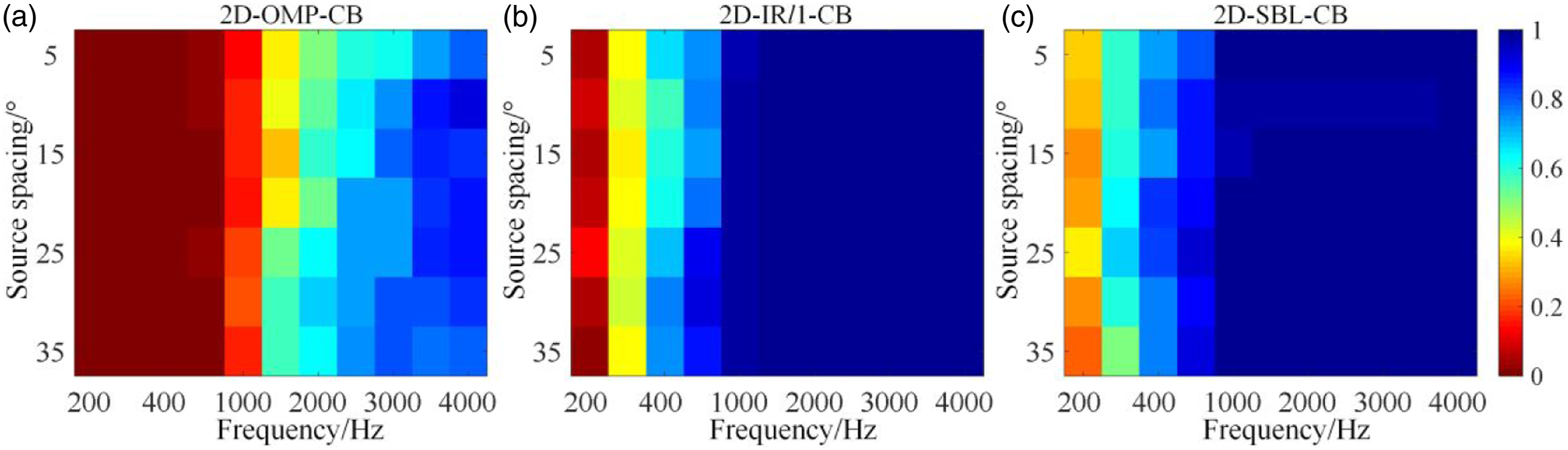
To explore the spatial resolution of the proposed method and generalize the conclusion, we performed the Monte–Carlo based simulations with different frequencies and source spacings. In these simulations, the grid spacing is set to $5°$ , source spacing is set to increase from $5°$ to $45°$ by 5° steps, and the frequency is set to 200, 300, 400, 500, 1000, 1500 ......4000 Hz. There are 11 × 9 = 99 combinations in total. We perform 100 trials for each combination. For each trial, we assume that there are two sources with equal strength and the same phase. The source strength ranges from 1 Pa to 2 Pa. The DOA of the source is on any grid point, while the source spacing and frequency are both certain values. Define the case where DOA estimate deviation $\partial$ is not greater than $1°$ as successful identification. Figure 6 shows the probability of successful identification $\text{CDF}\left(1°\right)$ obtained by the three CB methods with different frequencies and source spacings.

Figure 6.

The identification success probability $\text{CDF}\left(1°\right)$ of 2D-OMP-CB, 2D-IRl1-CB, and 2D-SBL-CB with different frequencies and source spacings.

As can be seen from Figure 6(a), when the source spacing is less than $20°$ , the identification success probability $\text{CDF}\left(1°\right)$ of 2D-OMP-CB is higher than 0.5 at frequencies not lower than 2000 Hz and increases with frequency. When the frequency is lower than 1000 Hz, the identification success probability $\text{CDF}\left(1°\right)$ of 2D-OMP-CB is close to 0 at different source spacings. Thus, the spatial resolution ability of 2D-OMP-CB is weak. From Figure 6(b), we can see that when the source spacing is in the range of $5°\sim 45°$ , the identification success probability $\text{CDF}\left(1°\right)$ of 2D-IRl1-CB is higher than 0.5 at frequencies not lower than 400 Hz and always close to 1 at frequencies higher than 1000 Hz, which indicates that 2D-IRl1-CB has significantly better spatial resolution than 2D-OMP-CB. In contrast, as shown in Figure 6(c), when the source spacing is in the range of $5°\sim 45°$ , the identification success probability $\text{CDF}\left(1°\right)$ of 2D-SBL-CB is always higher than 0.5 at frequencies not lower than 300 Hz. Even at 200 Hz, 2D-SBL-CB can still obtain an identification success probability $\text{CDF}\left(1°\right)$ of about 0.3, while 2D-IRl1-CB and 2D-OMP-CB can hardly successfully identify the sources ( $\text{CDF}\left(1°\right)$ is close to 0) in the same situation, which indicates that 2D-SBL-CB has better spatial resolution than 2D-IRl1-CB and far better than 2D-OMP-CB.

To explore the anti-interference performance of the proposed method, we performed the Monte–Carlo based simulations with different SNRs. Figure 7 shows the typical colormaps of three methods with the SNR of 5 dB and 2 dB. It can be seen from Figures 7(a)–(c) that when the SNR is 5 dB, both 2D-OMP-CB and 2D-SBL-CB can accurately identify all the sources, while 2D-IRl1-CB loses two sources and has inaccurate source strength quantification. When the SNR is 2 dB, 2D-IRl1-CB loses three sources and still has inaccurate source strength quantification. In contrast, both 2D-OMP-CB and 2D-SBL-CB can still accurately locate all the sources and only overestimate the strength of the weakest acoustic source. This is because when the SNR is 2 dB, the actual noise has exceeded the theoretical signal induced by the weak source, thus resulting in inaccurate strength quantification of the weakest source. These colormaps preliminarily show that 2D-SBL-CB and 2D-OMP-CB are less influenced by noise interference, and their anti-noise interference ability is better than that of 2D-IRl1-CB.

Figure 7.

The simulation colormaps of 2D-OMP-CB, 2D-IRl1-CB, and 2D-SBL-CB with SNR of 5 dB and 2 dB.

In addition, to further analyze the anti-noise interference ability of the proposed method and the influence of the number of snapshots, we performed the Monte–Carlo based simulations with different SNRs and snapshots. Figure 8 shows the probability of successful identification $\text{CDF}\left(1°\right)$ obtained by the three CB methods with different SNRs and the number of snapshots. Figure 9 shows the mean DOA estimation error ${\text{MAE}}_{\text{DOA}}$ and the mean source strength quantification error ${\text{MAE}}_{\text{Strength}}$ of the three CB methods for each case.

Figure 8.

The identification success probability CDF(1°) of 2D-OMP-CB, 2D-IRl1-CB, and 2D-SBL-CB with different SNRs and the number of snapshots.

Figure 9.

The mean direction of arrival estimation error and the mean source strength quantification error of 2D-OMP-CB, 2D-IRl1-CB, and 2D-SBL-CB with different signal-to-noise ratios and the number of snapshots.

As can be seen from Figure 8, when the SNR is higher than 20 dB, all three CB methods can obtain a high probability of successful identification, and 2D-SBL-CB and 2D-IRl1-CB have a slightly higher probability of successful source identification than that of 2D-OMP-CB. When the SNR is lower than 20 dB, 2D-IRl1-CB is heavily interfered with noise and can hardly identify the source with an extremely small probability of successful identification. In contrast, 2D-SBL-CB and 2D-OMP-CB suffer little noise interference, and their probability of successfully identifying the sound source only slightly decreases. The probability of successful identification of 2D-SBL-CB is still higher than that of 2D-OMP-CB.

Besides, from Figure 9, we can see that when the SNR is higher than 20 dB, ${\text{MAE}}_{\text{DOA}}$ of 2D-OMP-CB is about $0.03°$ with different number of snapshots, and ${\text{MAE}}_{\text{DOA}}$ of 2D-IRl1-CB and 2D-SBL-CB is close to $0°$ . As the SNR decreases, ${\text{MAE}}_{\text{DOA}}$ of the three CB methods also increases. When the SNR is 0 dB, ${\text{MAE}}_{\text{DOA}}$ of 2D-OMP-CB is about $0.12°$ at the snapshot number of 5, 2D-IRl1-CB can hardly identify the sources successfully, and ${\text{MAE}}_{\text{DOA}}$ of 2D-SBL-CB is about $0.06°$ at the snapshot number of 5. The 2D-SBL-CB has the highest accuracy of source identification, and ${\text{MAE}}_{\text{DOA}}$ is close to $0°$ with the increase of the number of snapshots. It can be seen that 2D-SBL-CB can obtain the highest probability of successful identification and highest accuracy of source identification among the three CB methods, regardless of the SNR, which indicates that 2D-SBL-CB has the strongest anti-noise interference ability.

Table 3 sums up the comprehensive performance of the proposed 2D-SBL-CB and the existing 2D-OMP-CB and 2D-IRl1-CB for acoustic source identification (more ★ indicates better performance). It can be seen that 2D-SBL-CB and 2D-IRl1-CB are insensitive to grid spacing and the acoustic source identification performance is relatively robust. The computational efficiency of 2D-SBL-CB and 2D-OMP-CB is significantly higher than that of 2D-IRl1-CB. In terms of spatial resolution, 2D-SBL-CB is the strongest, 2D-IRl1-CB is the second, and 2D-OMP-CB is the weakest. Besides, 2D-SBL-CB has the strongest anti-noise interference ability. Therefore, the comprehensive performance of the proposed 2D-SBL-CB is the best.

Table 3.

The comprehensive performance comparison of 2D-OMP-CB, 2D-IRl1-CB, and 2D-SBL-CB. CB = compressive beamforming; 2D = two-dimensional.

Comprehensive performance	2D-OMP-CB	2D-IRl1-CB	2D-SBL-CB
Robustness to grid spacing	★★	★★★	★★★
Computational efficiency	★★★	★	★★★
Spatial resolution	★	★★	★★★
Anti-noise interference ability	★★	★	★★★

CB = compressive beamforming; 2D = two-dimensional.

Conclusion

In this paper, we proposed a two-dimensional sparse Bayesian learning compressive beamforming (2D-SBL-CB). The proposed 2D-SBL-CB first assumes the signal prior and noise prior to derive the posterior probability distribution of the source strength and then adaptively estimates the hyperparameters of the sparse prior of source strength based on a type-II maximum likelihood, that is, by maximizing the evidence, to achieve source identification. Both simulations and experiment show that the proposed 2D-SBL-CB enjoys high computational efficiency, strong spatial resolution ability, and strong anti-noise interference. Besides, it is insensitive to grid spacing and has stable source identification performance. Compared with the existing 2D-OMP-CB and 2D-IRl1-CB, the proposed 2D-SBL-CB has the best comprehensive performance for acoustic source identification.