An approximation technique for solving nonlinear oscillators

Abstract

Recently, an approximation technique was presented for solving strong nonlinear oscillators modeled by second-order differential equations. Due to the arising of an algebraic complicity, the method fails to determine suitable solution of some important nonlinear problems such as quadratic oscillator, cubical Duffing oscillator of softening springs, and pendulum equation. However, suitable solutions of these oscillators are found by rearranging only an algebraic equation related to amplitude and frequency. The determination of solutions is simpler than the original version.

Introduction

The classical perturbation methods^1–5 were developed to investigate weakly nonlinear problems modeled by $\ddot{x}+{\omega }_0^{2}x+\epsilon f\left(x,\dot{x}\right)=0,$ (1)where $\epsilon \ll {\omega }_0^2$ . Herein, ${\omega }_0$ is known as the unperturbed frequency, $\epsilon$ is the constant, and $f$ is a nonlinear function. Then classical methods^6–9 were modified to overcome this limitation and applied to solve strong nonlinear problems, where $\epsilon =\mathrm{{\rm O}}\left(1\right)$ . On the other hand, some analytical techniques such as the homotopy perturbation method (HPM),^10–15 variational iteration method (VIM),^16–19 generalized homotopy method, ²⁰ harmonic balance method (HBM),^21,22 energy balance method (EBM),^23,24 and frequency–amplitude formula^25–27 were presented to solve equation (1) for $\epsilon =\mathrm{{\rm O}}\left(1\right)$ . Most of the above methods were developed based on trigonometric functions.

In 1986, Zhou ²⁸ first introduced a semi-analytical method named differential transform method (DTM) in which the solution is chosen as a truncated Maclaurin series and applied to analyze linear and nonlinear electric circuit problems. Then some authors applied the DTM^29–34 to solve linear and nonlinear differential equations. But such truncated series solution does not nicely exhibit the periodic behavior which is characteristic of oscillator equations. It provides satisfactory results within a small region only. In order to improve the accuracy of the DTM, an alternative technique was used which modifies the series solution for nonlinear oscillatory systems. A modification of the DTM, based on the use of Padé approximants, was proposed by Shahed ³⁵ for solving different types of nonlinear problems. Further, Momani et al., ³⁶ Nourazar et al., ³⁷ and Benhammouda et al. ³⁸ modified the DTM by applying the Laplace–Padé resummation method. However, it is a laborious task.

Recently, Alam et al. ³⁹ presented an analytical technique for solving equation (1). But the method ³⁹ is useless for some nonlinear oscillators such as quadratic oscillator (in region $x<0$ ), cubical oscillator of softening springs (i.e., Duffing equation, $\ddot{x}+{\omega }_0^{2}x+\epsilon x^3=0$ , $\epsilon <0$ ), and pendulum equation. The aim of this article is to find suitable solutions for these situations. Moreover, the solution (concern of this article) provides desired results for a wide variety of nonlinear oscillators whether $f\left(-x,-\dot{x}\right)=-f\left(x,\dot{x}\right)$ or not. Thus, the method also covers the cases of quadratic oscillator (in region $x>0$ ), cubical oscillator of hardening springs (Duffing equation, $\epsilon >0$ ), etc.

The method

By variable transformation, $\tau =\omega t$ , equation (1) with initial conditions $\left[x\left(0\right)=0,\dot{x}\left(0\right)=b\right]$ becomes ${\omega }^2{x}^{″}+{\omega }_0^{2}x+\epsilon f\left(x,\omega x^{\prime }\right)=0;\hspace{0.17em}x\left(0\right)=0,x^{\prime }\left(0\right)=\frac{b}{\omega }=\beta ,$ (2)where primes denote differentiation with respect to $\tau$ . In general, initial conditions are chosen as $x\left(0\right)=a,\dot{x}\left(0\right)=0$ , but in Ref. ³⁹ , the former conditions were considered.

A polynomial type of solution of $\phi =\tau \left(\pi -\tau \right)$ of equation (2) was found in a form ³⁹ $x\left(\tau \right)=B_1\left(\beta ,{\omega }_0,\epsilon ,\omega \right)\phi \left(\tau \right)+B_2\left(\beta ,{\omega }_0,\epsilon ,\omega \right){\phi \left(\tau \right)}^2+B_3\left(\beta ,{\omega }_0,\epsilon ,\omega \right){\phi \left(\tau \right)}^3+\dots ,$ (3)when $f\left(-x,-\dot{x}\right)=-f\left(x,\dot{x}\right)$ . Solution equation (3) is also valid when $f\left(-x,-\dot{x}\right)=f\left(x,\dot{x}\right)$ . It is obvious that equation (3) satisfies the first initial condition given in equation (2). Usually, solution equation (3) is used for a semi-period of oscillation, $0<\tau \le \pi$ . For the next semi-period, $\phi$ and $\beta$ are changed, respectively, by $\phi =\left(\tau -\pi \right)\left(2\pi -\tau \right)$ , $\pi \le \tau \le 2\pi$ , and $–\beta$ . Substituting equation (3) into equation (2) and then equating coefficients of ${{\phi }^0,\phi }^1,{\phi }^2,{\phi }^3,\cdots$ , a set of linear algebraic equations of $B_i,i=1,2,3,\cdots$ are obtained whose solution provides the noted unknown coefficients. The value of $x\left(\tau \right)$ has the maximum value (known as amplitude of oscillation, say $a>0$ ) at $\tau =\pi /2$ . Therefore, a relation between amplitude and frequency becomes $a=\frac{B_1\left(\beta ,{\omega }_0,\epsilon ,\omega \right){\pi }^2}{4}+\frac{B_2\left(\beta ,{\omega }_0,\epsilon ,\omega \right){\pi }^4}{16}+\frac{B_3\left(\beta ,{\omega }_0,\epsilon ,\omega \right){\pi }^6}{64}+\cdots .$ (4)

On the other hand, $x\left(\tau \right)$ has the minimum value (say $-a*$ ) at $\tau =3\pi /2$ . In this case, $\beta$ can be replaced by $–\beta$ and $\omega$ by $\omega *$ . Therefore, equation (4) is replaced by $-a*=\frac{B_1\left(-\beta ,{\omega }_0,\epsilon ,\omega *\right){\pi }^2}{4}+\frac{B_2\left(-\beta ,{\omega }_0,\epsilon ,\omega *\right){\pi }^4}{16}+\frac{B_3\left(-\beta ,{\omega }_0,\epsilon ,\omega *\right){\pi }^6}{64}+\cdots .$ (5)when $f\left(-x,-\dot{x}\right)=-f\left(x,\dot{x}\right)$ , $a*=a$ , and equation (4) and equation (5) are identical. So, $\omega =\omega *$ . However, a problem arises when $f\left(-x,-\dot{x}\right)=f\left(x,\dot{x}\right)$ . In this case, $a*$ and $a$ have different values. For this reason, $\omega$ and $\omega *$ have different values. Usually $a$ is given and $a*$ is determined. Therefore, an algebraic relation is required between $a$ and $a*$ . Moreover, equation (4) contains two unknown $\beta$ and $\omega$ , and equation (5) contains $\beta$ and $\omega *$ . Therefore, it requires another relation involving them.

Now multiplying both sides of equation (2) by $2x^{\prime }$ and then integrating with respect to $\tau$ ${{\omega }^2{x}^{\prime }}^2+G\left(x,{\omega }_0,\epsilon \right)=C,$ (6)where $G\left(x,{\omega }_0,\epsilon \right)=2\int {(\omega }_0^{2}x+\epsilon f\left(x\right))dx$ when $f$ is a function of $x$ only and $C$ is an integration constant. It has already been mentioned that $x\left(\tau \right)$ is the maximum at $\tau =\pi /2$ and minimum at $\tau =3\pi /2$ . So, $x^{\prime }$ vanishes at these limits. On the other hand, $x$ as well as $G\left(x,{\omega }_0,\epsilon \right)$ vanishes at $\tau =0$ and $\tau =\pi$ . At these limits, $x^{\prime }$ , respectively, becomes $\beta$ and $–\beta$ . Thus, the following relations are obtained from equation (6). $G\left(a,{\omega }_0,\epsilon \right)={\omega }^2{\beta }^2.$ (7)and $G\left(-a*,{\omega }_0,\epsilon \right)={\omega }^2{\beta }^2.$ (8)Comparing equation (7) and equation (8), the relation between $a$ and $a*$ is obtained as $G\left(-a*,{\omega }_0,\epsilon \right)=G\left(a,{\omega }_0,\epsilon \right).$ (9)

Finally, solving equation (4) and equation (7), $\beta$ and $\omega$ are obtained. In a similar way, $\beta$ and $\omega *$ are obtained solving equation (5) and equation (8).

Examples

Duffing (cubical) oscillator

Let us consider the Duffing oscillator $\ddot{x}+{\omega }_0^{2}x+\epsilon x^3=0,x\left(0\right)=0,\dot{x}\left(0\right)=b.$ (10)

Substituting solution equation (3) into equation (10) and then equating the coefficients of ${\phi }^0$ , ${\phi }^1,{\phi }^2,{\phi }^3,\cdots$ , the following algebraic equations are derived: $B_1-B_2{\pi }^2=0,$ ${{\omega }_0^{2}B}_1-12{{\omega }^{2}B}_2+6{\pi }^2{\omega }^2{B}_3=0,$ $\epsilon B_1^2+{{\omega }_0^{2}B}_2-30{{\omega }^{2}B}_3+12{\pi }^2{\omega }^2{B}_4=0,\cdots$ (11)

Solving equation (11), the unknown coefficients are derived as $B_2=\frac{B_1}{{\pi }^2},B_3=-\frac{{{\omega }_0^{2}B}_1}{6{\pi }^2{\omega }^2}+\frac{2B_2}{{\pi }^2},B_4=-\frac{{{\omega }_0^{2}B}_2}{12{\pi }^2{\omega }^2}+\frac{5B_3}{2{\pi }^2}-\frac{\epsilon B_1^2}{12{\pi }^2{\omega }^2},\cdots$ (12)Now, differentiating equation (3) with respect to $\tau$ and then substituting $\tau =0$ (i.e., by utilization of the second initial condition), it becomes $x^{\prime }\left(0\right)=\beta =\pi B_1$ (13)Now, from equation (12) and equation (13), all unknown coefficients can be written in terms of $\beta$ as ${B_1=\frac{\beta }{\pi },B}_2=\frac{\beta }{{\pi }^3},B_3=-\frac{{\omega }_0^2\beta }{6{\pi }^3{\omega }^2}+\frac{2\beta }{{\pi }^5},B_4=\frac{5\beta }{{\pi }^7}-\frac{{\omega }_0^2\beta }{2{\pi }^5{\omega }^2},\cdots$ (14)Substituting these values of unknown coefficients (up to ${\mathrm{B}}_{10}$ ) in equation (4), it becomes $a=\frac{\beta \pi }{4}\left(1+\frac{1}{4}+\frac{1}{8}\cdots +\frac{2431}{131072}\right)-\frac{\beta {\pi }^3{\omega }_0^2}{384{\omega }^2}\left(1+\frac{3}{4}+\frac{9}{16}+\cdots +\frac{429}{2048}\right)$ $+\left(\frac{\beta {\pi }^5{\omega }_0^4}{122880{\omega }^4}-\frac{{\beta }^3{\pi }^5\epsilon }{20480{\omega }^2}\right)\left(1+\frac{5}{4}+\cdots +\frac{1001}{1024}\right)-\left(\frac{\beta {\pi }^7{\omega }_0^6}{82575360{\omega }^6}-\frac{{11\beta }^3{\pi }^7{\omega }_0^2\epsilon }{13762560{\omega }^4}\right)\left(1+\frac{7}{4}+\cdots +\frac{77}{32}\right)$ $+\left(\frac{\beta {\pi }^9{\omega }_0^8}{95126814720{\omega }^8}-\frac{17{\beta }^3{\pi }^9{\omega }_0^4\epsilon }{2642411520{\omega }^6}+\frac{{\beta }^5{\pi }^9{\epsilon }^2}{125829120{\omega }^4}\right)\left(1+\frac{9}{4}\right).$ (15)or $a=\frac{215955\mathrm{\beta }\pi }{524288}-\frac{15751\mathrm{\beta }{\pi }^3{\omega }_0^2}{1572864{\omega }^2}+\frac{459\mathrm{\beta }{\pi }^5{\omega }_0^4}{8388608{\omega }^4}-\frac{1377{\mathrm{\beta }}^3{\pi }^5\epsilon }{4194304{\omega }^2}+\frac{517{\mathrm{\beta }}^3{\pi }^7\epsilon {\omega }_0^2}{88080384{\omega }^4}-\frac{47\mathrm{\beta }{\pi }^7{\omega }_0^6}{528482304{\omega }^6}$ $+\frac{13\mathrm{\beta }{\pi }^9{\omega }_0^8}{380507258880{\omega }^8}-\frac{221{\mathrm{\beta }}^3{\pi }^9\epsilon {\omega }_0^4}{10569646080{\omega }^6}+\frac{13{\mathrm{\beta }}^5{\pi }^9{\epsilon }^2}{503316480{\omega }^4}$ (16)

For this oscillator, equation (7) becomes ${{\omega }^2{\beta }^2=\omega }_0^2{a}^2+\frac{\epsilon a^4}{2}$ (17)and it can be written as $$\beta =\frac{a\eta }{\mathrm{\omega }},\mathrm{w}\mathrm{h}\mathrm{e}\mathrm{r}\mathrm{e}\hspace{0.17em}\eta =\sqrt{\left({\omega }_0^2+\frac{\epsilon a^2}{2}\right)}$$ (18)By substitution of $\omega =a\hspace{0.17em}\eta /\beta$ in equation (16), it becomes $\beta =\frac{a}{\left(\frac{215955\pi }{524288}+\frac{13{\beta }^4{\pi }^9{\epsilon }^2}{503316480a^4{\eta }^4}-\frac{1377{\beta }^2{\pi }^5\epsilon }{4194304a^2{\eta }^2}+\frac{517{\beta }^2{\pi }^7\epsilon {\omega }_0^2}{88080384a^4{\eta }^4}-\frac{15751{\pi }^3{\omega }_0^2}{1572864a^2{\eta }^2}-\frac{221{\beta }^2{\pi }^9\epsilon {\omega }_0^4}{10569646080a^6{\eta }^6}+\frac{459{\pi }^5{\omega }_0^4}{8388608a^4{\eta }^4}-\frac{47{\pi }^7{\omega }_0^6}{528482304a^6{\eta }^6}+\frac{13{\pi }^9{\omega }_0^8}{380507258880a^8{\eta }^8}\right)}$ (19)When $a$ is given, the value of $\beta$ is obtained from equation (19) by an iterative procedure, starting with initial ${\beta }_0=a$ . Therefore, the solution of Duffing oscillator equation (10) is obtained from equation (3) by substituting the values of $B_1,B_2,\cdots ,B_{10}$ from equation (14).

Quadratic oscillator

Let us consider the quadratic oscillator $\ddot{x}+{\omega }_0^{2}x+\epsilon x^2=0,x\left(0\right)=0,\dot{x}\left(0\right)=b$ (20)

For this oscillator, unknown coefficients have been obtained: ${B_1=\frac{\beta }{\pi },B}_2=\frac{\beta }{{\pi }^3},B_3=-\frac{{\omega }_0^2\beta }{6{\pi }^3{\omega }^2}+\frac{2\beta }{{\pi }^5},B_4=-\frac{{\omega }_0^2\beta }{2{\pi }^5{\omega }^2}+\frac{5\beta }{{\pi }^7}-\frac{\epsilon {\beta }^2}{12{\pi }^4{\omega }^2},\cdots$ (21)Substituting these values of unknown coefficients (up to ${\mathrm{B}}_9$ ) in equation (4), it becomes $a=\frac{53381\beta \pi }{131072}+\frac{\beta {\pi }^9{\omega }_0^4}{95126814720{\omega }^8}-\frac{79\beta {\pi }^7{\omega }_0^3}{1321205760{\omega }^6}-\frac{{\beta }^2{\pi }^8{\omega }_0^2\epsilon }{20971520{\omega }^6}-\frac{5{\beta }^3{\pi }^9{\omega }_0{\epsilon }^2}{1585446912{\omega }^6}+\frac{1471\beta {\pi }^5{\omega }_0^2}{3145\mathrm{\gamma }7280{\omega }^4}+\frac{21{\beta }^2{\pi }^6{\omega }_0\epsilon }{1048576{\omega }^4}+\frac{79{\beta }^3{\pi }^7{\epsilon }^2}{66060288{\omega }^4}-\frac{14893\beta {\pi }^3{\omega }_0}{1572864{\omega }^2}-\frac{103{\beta }^2{\pi }^4\hspace{0.17em}\epsilon }{65536{\omega }^2}$ (22)

For this oscillator, equation (7) becomes ${{\omega }_0^{2}a}^2+\frac{2ϵa^3}{3}={\omega }^2{\beta }^2$ (23)and it can be written as $$\beta =\frac{a\eta }{\mathrm{\omega }},\mathrm{w}\mathrm{h}\mathrm{e}\mathrm{r}\mathrm{e}\hspace{0.17em}\eta =\sqrt{\left({\omega }_0^2+\frac{2\epsilon a}{3}\right)}$$ (24)By substitution of $\omega =a\hspace{0.17em}\eta /\beta$ in equation (22), it becomes $\beta =\frac{a}{\left(\frac{53381\pi }{131072}+\frac{{\beta }^8{\pi }^9{\omega }_0^4}{95126814720a^8{\eta }^8}-\frac{79{\beta }^6{\pi }^7{\omega }_0^3}{1321205760a^6{\eta }^6}+\frac{1471{\beta }^4{\pi }^5{\omega }_0^2}{31457280a^4{\eta }^4}-\frac{14893{\beta }^2{\pi }^3{\omega }_0}{1572864a^2{\eta }^2}-\frac{{\beta }^7{\pi }^8\epsilon \hspace{0.17em}{\omega }_0^2}{20971520a^6{\eta }^6}+\frac{21{\beta }^5{\pi }^6\epsilon {\omega }_0}{1048576a^4{\eta }^4}-\frac{103{\beta }^3{\pi }^4\epsilon }{65536a^2{\eta }^2}-\frac{5{\beta }^8{\pi }^9{\epsilon }^2}{1585446912a^6{\eta }^6}+\frac{79{\beta }^6{\pi }^7{\epsilon }^2}{66060288a^4{\eta }^4}\right)}$ (25)When $a$ is given, the value of $\beta$ is obtained from equation (25) by an iterative procedure, starting with initial ${\beta }_0=a$ . For the next semi-period, corresponding equation (24) and equation (25) become $\beta *=\frac{a*\eta *}{\omega *},\mathrm{w}\mathrm{h}\mathrm{e}\mathrm{r}\mathrm{e}\hspace{0.17em}\eta *=\frac{\sqrt{{\omega }_0^2-2\epsilon a*}}{3}$ (26) ${-\beta }^{*}=\frac{-a*}{\left(\frac{53381\pi }{131072}+\frac{{(\beta *)}^8{\pi }^9{\omega }_0^4}{95126814720{(a*)}^8{(\eta *)}^8}-\frac{79{(\beta *)}^6{\pi }^7{\omega }_0^3}{1321205760{(a*)}^6{(\eta *)}^6}+\frac{1471{(\beta *)}^4{\pi }^5{\omega }_0^2}{31457280{(a*)}^4{(\eta *)}^4}-\frac{14893{(\beta *)}^2{\pi }^3{\omega }_0}{1572864{(a*)}^2{(\eta *)}^2}+\frac{{(\beta *)}^7{\pi }^8\epsilon \hspace{0.17em}{\omega }_0^2}{20971520{(a*)}^6{(\eta *)}^6}-\frac{21{(\beta *)}^5{\pi }^6\epsilon {\omega }_0}{1048576{(a*)}^4{(\eta *)}^4}+\frac{103{(\beta *)}^3{\pi }^4\epsilon }{65536{(a*)}^2{(\eta *)}^2}-\frac{5{(\beta *)}^8{\pi }^9{\epsilon }^2}{1585446912{(a*)}^6{(\eta *)}^6}+\frac{79{(\beta *)}^6{\pi }^7{\epsilon }^2}{66060288{(a*)}^4{(\eta *)}^4}\right)}$ (27)where $a*=\left(3+2\epsilon a-\sqrt{3-4\epsilon a-4a^2{\epsilon }^2}\right)/4\epsilon$ .

When $a*$ is given, the value of ${\beta }^{*}$ is obtained from equation (27) by an iterative procedure, starting with initial ${\beta }_0^{*}=a*$ . Therefore, the solution of quadratic oscillator equation (20) is obtained from equation (3) by substituting the values of $B_1,B_2,\cdots ,B_9$ from equation (21).

Pendulum equation

Let us consider the pendulum equation $\ddot{x}+\sin \hspace{0.17em}x=0,\hspace{1em}x\left(0\right)=0,\hspace{1em}\dot{x}\left(0\right)=b$ (28)

For this oscillator, unknown coefficients have been obtained: ${B_1=\frac{\beta }{\pi },B}_2=\frac{\beta }{{\pi }^3},B_3=-\frac{\beta }{6{\pi }^3{\omega }^2}+\frac{2\beta }{{\pi }^5},B_4=\frac{5\beta }{{\pi }^7}-\frac{\beta }{2{\pi }^5{\omega }^2},\cdots$ (29)Substituting these values of unknown coefficients (up to ${\mathrm{B}}_{10}$ ) in equation (4), it becomes $a=\frac{215955\beta \pi }{524288}+\frac{13\beta {\pi }^9}{380507258880{\omega }^8}-\frac{47\beta {\pi }^7}{528482304{\omega }^6}+\frac{221{\beta }^3{\pi }^9}{63417876480{\omega }^6}+\frac{459\beta {\pi }^5}{8388608{\omega }^4}-\frac{517{\beta }^3{\pi }^7}{528482304{\omega }^4}+\frac{247{\beta }^5{\pi }^9}{126835752960{\omega }^4}-\frac{15751\beta {\pi }^3}{1572864{\omega }^2}+\frac{459{\beta }^3{\pi }^5}{8388608\hspace{0.17em}{\omega }^2}-\frac{47{\beta }^5{\pi }^7}{528482304{\omega }^2}+\frac{13{\beta }^7{\pi }^9}{380507258880{\omega }^2}$ (30)

For this oscillator, equation (7) becomes ${\omega }^2{\beta }^2=2\left(1-\cos \hspace{0.17em}a\right)$ (31)and it can be written as $\beta =\frac{\eta }{\mathrm{\omega }},\eta =\sqrt{2\left(1-\cos \hspace{0.17em}a\right)}$ (32)By substitution of $\omega =\eta /\beta$ in equation (30), it becomes $\beta =\frac{a}{\left(\frac{215955\pi }{524288}+\frac{13{\beta }^8{\pi }^9}{380507258880{\eta }^8}-\frac{47{\beta }^6{\pi }^7}{528482304{\eta }^6}+\frac{221{\beta }^8{\pi }^9}{63417876480{\eta }^6}+\frac{459{\beta }^4{\pi }^5}{8388608{\eta }^4}-\frac{517{\beta }^6{\pi }^7}{528482304{\eta }^4}+\frac{247{\beta }^8{\pi }^9}{126835752960{\eta }^4}-\frac{15751{\beta }^2{\pi }^3}{1572864{\eta }^2}+\frac{459{\beta }^4{\pi }^5}{8388608{\eta }^2}-\frac{47{\beta }^6{\pi }^7}{528482304{\eta }^2}+\frac{13{\beta }^8{\pi }^9}{380507258880{\eta }^2}\right)}$ (33)When $a$ is given, the value of $\beta$ is obtained from equation (33) by an iterative procedure, starting with initial ${\beta }_0=a$ . Therefore, the solution of pendulum equation (28) is obtained from equation (3) by substituting the values of $B_1,B_2,\cdots ,B_{10}$ from equation (29).

Results and discussion

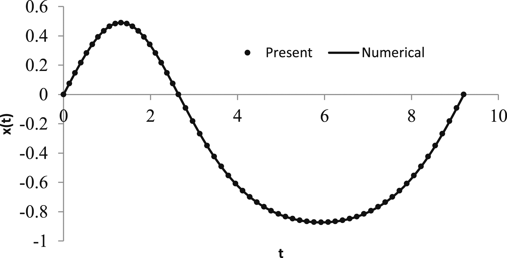
In this section, solutions for various nonlinear oscillators obtained by the present method are compared with corresponding numerical solutions (4th-order Runge–Kutta method). First of all, solutions of the Duffing oscillator for different initial conditions are presented in Figures 1–5. From these figures, it is clear that present solutions agree with corresponding numerical solutions whether $\epsilon <0$ or $\epsilon >0$ . It is noted that a solution of the Duffing equation exists for all values of $a$ when $\epsilon >0$ . On the contrary, a periodic solution of this oscillator is found for some particular values of $a$ when $\epsilon <0$ (e.g., $a<1$ when $\epsilon =-1$ ).

Figure 1.

Comparison of the solutions between the present method and the numerical method for the Duffing oscillator with the initial condition [ $x\left(0\right)=0,\dot{x}\left(0\right)=0.659696900988258$ ] for ${\omega }_0=1$ and $\epsilon =-1$ , where $a=0.8$ .

Figure 2.

Comparison of the solutions between the present method and the numerical method for the Duffing oscillator with the initial condition [ $x\left(0\right)=0,\dot{x}\left(0\right)=0.679335612933695$ ] for ${\omega }_0=1$ and $\epsilon =-1$ , where $a=0.85$ .

Figure 3.

Comparison of the solutions between the present method and the numerical method for the Duffing oscillator with the initial condition [ $x\left(0\right)=0,\dot{x}\left(0\right)=0.6942261879243681$ ] for ${\omega }_0=1$ and $\epsilon =-1$ , where $a=0.9$ .

Figure 4.

Comparison of the solutions between the present method and the numerical method for the Duffing oscillator with the initial condition [ $x\left(0\right)=0,\dot{x}\left(0\right)=71.4142842854285$ ] for ${\omega }_0=1$ and $\epsilon =1$ , where $a=10$ .

Figure 5.

Comparison of the solutions between the present method and the numerical method for the Duffing oscillator with the initial condition [ $x\left(0\right)=0,\dot{x}\left(0\right)=283.5489375751565$ ] for ${\omega }_0=1$ and $\epsilon =1$ , where $a=20$ .

For the quadratic oscillator, the solutions agree with numerical solutions for different values of $a\epsilon <1/2$ . In Figures 6 and 7, respectively, for $a=0.49$ and $a=0.495$ , the solutions are presented together with corresponding numerical solutions when $\epsilon =1$ .

Figure 6.

Comparison of the solutions between the present method and the numerical method for the quadratic oscillator with the initial condition [ $x\left(0\right)=0,\dot{x}\left(0\right)=0.564386983076919$ ] for ${\omega }_0=1$ and $\epsilon =1$ , where $a=0.49$ .

Figure 7.

Comparison of the solutions between the present method and the numerical method for the quadratic oscillator with the initial condition [ $x\left(0\right)=0,\dot{x}\left(0\right)=0.5708618484362044$ ] for ${\omega }_0=1$ and $\epsilon =1$ , where $a=0.495.$

In Figures 8 and 9, for $a=2.0$ and $a=2.25$ , solutions of the pendulum equation are presented together with numerical solutions. The periodic solution of this oscillator is found for all values of $a<\pi$ . But it requires a lot of terms of $\phi$ when $a\approx 3$ . On the other hand, it requires many harmonic terms to obtain a desired result by the homotopy perturbation method or VIM or harmonic balance method, etc., when $a\approx 3$ .

Figure 8.

Comparison of the solutions between the present method and the numerical method for the pendulum equation with the initial condition [ $x\left(0\right)=0,\dot{x}\left(0\right)=1.682941969615793$ ] for $a=2.0$ .

Figure 9.

Comparison of the solutions between the present method and the numerical method for the pendulum equation with the initial condition [ $x\left(0\right)=0,\dot{x}\left(0\right)=1.8045351881981904$ ] for $a=2.25.$

It is noted that the homotopy perturbation method, VIM, harmonic balance method, etc., are widely used tools for handling strong nonlinear oscillators. But every method has some limitations. The homotopy perturbation method provides good results for the Duffing oscillator; but it is useless for the quadratic oscillator when $a\epsilon \approx 1/2$ (Appendix B). The advantage of the present method is that it nicely covers both oscillators.

Conclusion

An approximation technique is presented for solving various strongly nonlinear oscillators. The determination of a solution is simpler than its original version. The trial solution is completely algebraic and the coefficients of unknown variables are determined by solving a set of simple linear equations. The method is similar to the DTM, but it is much easier.