Sage Journals: Discover world-class research

Abstract

Event sequence data consists of discrete events that happen over time. By grouping events based on common entities and ordering them chronologically, they form sequences. Events are registered in different domains, ranging from healthcare to logistics. Collections of these sequences typically represent high-level processes for users to discover, identify, and analyze. This discovery is challenging, given that sequences in real-world scenarios can grow long, have many events, many attribute dimensions of events, and/or various event categories. However, limited research focuses on analyzing long event sequences, the focus of this paper. We present LoLo, an interactive visual analytics method based on the analysis of multi-level structures in long event sequence collections. LoLo introduces a strategy to split the sequence collection into meaningful data-driven stages, where the definition of a stage facilitates interpretation and injection of domain knowledge. The stages have different levels, which represent high-level processes taking into account high-level changes (global staging) combined with local sequence variations (local staging). We demonstrate the effectiveness of LoLo by comparing it to a baseline and present two use cases, one is evaluated with two users and the other by us, on real-world data sets showing that our staging method can capture the semantic content in stages and users appreciate being able to switch between different levels of detail.

Keywords

visual analytics visualization event sequence data scalability staging

Introduction

Process data changing over time is often recorded as discrete event sequences in various domains. An event represents an occurrence of a discrete activity with one or multiple multivariate attributes in addition to an id, timestamp, and optionally a duration. Events having only a single attribute besides id, timestamp, and duration, are called univariate events. Events are grouped into chronologically ordered sequences based on entities (referred to as cases). Due to ever-growing event data collections, current visual analytics methods focus on several scalability aspects. Scalability can relate to events, for example, thousands of event types¹ or events with more than 70 attributes.² In other contexts, scalability relates to the sequences, for example, many sequences³ or long sequences. However, while omnipresent, there is little work on scalable visual analytics methods for long sequences, which is the focus of this paper. We define long as a sequence with more than a thousand events, in line with the definition of the state-of-the-art of Van der Linden et al.⁴ We opted for at least a thousand events because conventional visualization and computational methods, such as visualizing all events as blocks, fail, for example, take too long or cannot display all the elements on the screen which leads to scrolling. Many domains register events with well over thousands of events, for example, healthcare - the MIMIC dataset,⁵ security,⁶ governance - neighborhood complaints,⁷ and genomics data.

A collection of long event sequences typically contains a shared high-level event structure, for example, processes in a hospital, with events grouped by patient or doctor. This structure can be a set of stages, subsequences with shared characteristics that are not known in advance. Our aim is to discover these stages on different levels of abstraction. Different levels are needed to be able to keep the details but at the same time have a meaningful structure. Once multiple stages are defined, it is interesting why they transition from one stage to another and if stages are repeated in time. This reveals high-level structures that are interesting for a global understanding of the underlying process. Especially in long sequences, the probability of small deviations in event patterns is high. These small, detailed deviations of specific patterns (e.g., exact matching patterns) are less interesting for understanding this high-level structure of the progression of the process.⁸ In the related field of visualization of genome data, we find additional examples for visualizing long sequences as surveyed by Nusrat et al.⁹ However, to our knowledge, the goal is not to identify semantically repeated stages over time, which is our goal, but rather to focus more on specific patterns of events, for example, genes. Another related field studying event sequences is process mining, however, they do not focus on the interactive visualization, but rather on algorithmic development.

The derived multi-level stages differ in duration and, therefore, subsequence length. Understanding the underlying high-level structures by discovering stages from different abstraction levelsallows to verify if cases are treated consistently in the system, for example, hospital patients, factory products, etc. The factors that influence the quality of a discovered stage depend on the domain and the specific user query in mind. Therefore, users need to understand the stages on different aggregation levels, for example, hierarchically, and be able to interactively explore, validate, and adapt them based on their domain knowledge.

State-of-the-art event sequence visualizations often focus on detailed, low-level patterns¹⁰ or the stages are constructed based on fixed time windows, for example, the work of Guo et al.¹¹ Fixed windows segment the sequences in subsequences by using a fixed time period or number of events to create the stages rather than building stages that are semantically meaningful or have shared events/patterns. For example, in the hospital emergency department, patients are treated differently and their treatment duration can differ drastically. The sequences of these different patients cannot be clearly split using fixed time windows. The context and event labels are ignored using this splitting method, and the split can occur in the middle of a treatment. Also, the semantically similar time periods, (a set of) treatments and medications treating the same (phase of a) disease, are not known upfront and differ in length. Closest to our research is another work by Guo et al.⁸ that with a maximum average sequence length of approximately 800. However, the subdivision method is rather black box using methods from the text analysis field and ground truth information on stages is typically unavailable. This hinders the interpretation of the discovered stages, which is important to be able to use the results of the stages. Whether the methods focus on low-level patterns or high-level structures, visualizations, for example, Sequen-C³ or Guo et al.,⁸ have visual⁸ and computational^3,8 scalability challenges. This hampers the visualization of long sequences and the interactive injection of domain knowledge to adapt the stages in the staging algorithms, respectively. Interactive visualization of those stages is needed to explore and discover the high-level structures.

We present LoLo, a domain-independent interactive visual analytics method to analyze long univariate event sequences. It considers long sequences, which contain a lot of events and insights, hence the name LoLo. Our contributions are:

a strategy to discover stages that allow for semantic interpretation and interactive refinement based on users’ domain knowledge; and,

a visual analytics approach to analyze the multi-level structure of long event sequences by identifying hierarchical stages.

The paper is structured as follows: first, we identify tasks for analyzing long sequences and related work. Second, we describe the stage generation and visualization. Third, using two real-world data sets, we evaluate LoLo with two experts and present a discussion and conclusions.

User tasks

We identify which tasks are most relevant when dealing with long sequences. Our target user group is data analysts/researchers working with long sequence data in different domains, such as healthcare, security, and energy. We analyzed and identified user tasks based on tasks and challenges from papers mentioned in related work, and additionally, discussions between the authors experienced with event sequence visualization.

T1 Interactively (re)define stages based on domain knowledge. To utilize users’ domain knowledge and address that there is no ground truth, users need to be able to adjust the stages to explore the effects of different parameters based on their domain knowledge. This is based on Guo et al.¹¹

T2 Identify (reoccurring and outlier) stages over time. To get an overview of the high-level structure of long sequences. Stages summarize the long event sequences that contain too much data and variety to analyze without aggregation. Which (ordering of) events contributed to the resulting stages should be presented and explained clearly to users. Users need to interpret the stages and identify which behaviors/stages are repeated over time. Outlier stages, that is, events (orderings) differ from surrounding stages or the order of stages with certain characteristics differ, are possible indicators of disturbances in the process. This task is based on Guo et al.⁸ and Wang et al.¹²

T3 Compare and group similar stages. Users want to compare different stages over time to observe their similarity to identify the main characteristics of the different stages discovered and where similar stages reoccur over time. This is still on a higher level of abstraction, which should be explainable (users should understand why these stages are formed by the algorithm) to users because comparing similarities is not straightforward due to subsequences in stages often still being long. This task is based on Guo et al.^8,11 and Wang et al.¹³

T4 Understand transitions between stages. Users need to know why the sequences progress from one stage to another. They want to understand the transition of consecutive stages. When dealing with long sequences these transitions could also contain subsequences of hundreds of events or more, so explainable abstractions are needed. This task is based on Wang et al.¹² and Guo et al.⁸

T5 Understand the hierarchical stage structure and switch between aggregated stages and detailed sequence and event information. To explain why stages are discovered, it is essential to have low-level details and aggregations with different levels of abstraction. These abstractions either abstract complete stages in a hierarchical structure or abstract subsequences within a stage. Users should not be overwhelmed by the long (sub)sequences. This task is inspired by Guo et al.¹⁴ and Chen et al.¹⁵ It can be combined with T3 and T4 to get a detailed, multi-level understanding of stage similarities and transitions.

Related work

In general, researchers and domain experts perform several main tasks when analyzing event sequence data, such as comparison⁴ (similar to T3) and summarization¹⁴ (similar to T2). Users execute these tasks on data of varying sizes which typically influence the analysis process. For example, a large number (more than a thousand) of sequences,^1,3,13,16,17 a large number (more than a thousand) of categories,¹ a large number (more than 50) of attributes,² or long (more than a thousand events) sequences.¹³ Data reduction strategies help reduce data variety and volume.¹⁸ To go into more detail of discovering stages and visualizing them in long sequences, we first describe an overview of related work regarding finding and analyzing high-level structures, for example, stages, in event sequence collections. Second, we discuss related work visualizing those.

High-level structure identification

As mentioned in the introduction, there are low-level, exact matching patterns, typically found using frequent pattern mining, and high-level structures. We focus on methods to find high-level structures through fixed or dynamic staging.

Fixed staging is the most common approach, also present in related fields, such as network visualization, where methods use fixed time intervals to discover stages.^11,19,20 However, the process underpinning the sequences is not always bound to fixed time intervals, for example, emergency treatments in a hospital. Fixed time intervals likely cause sequences to be cut in the middle of their high-level structure. A sliding-window approach²⁰ partially solves this, but still there is the challenge on how to define the window size.

With dynamic staging, that is, stages based on the event sequence data and not a predefined time-span, there are solely non-interactive black box machine learning methods such as hierarchical clustering²¹ or coordinate ascent strategy/expectation-maximization algorithms²² to discover stages. It is difficult to interpret and reason about the resulting stages.¹¹ On the other hand, there are interactive visual methods. DPVis²³ provides a visual analytics methods to discover states using hidden Markov models and aim for interpretability. However, in their approach, they discover states, that is, each multivariate event is given a classification, instead of segmenting a sequence collection in stages (our aim). Chen et al.¹⁵ construct a hierarchical visualization based on frequent patterns, having multiple hierarchical visualizations to describe the entire data set. It is hard to capture the high-level structure of the entire collection (T2 and T5), because identifying where in time the patterns of different hierarchies occur is not straightforward. Moreover, when the length of the sequences increases, the hierarchical trees become large. Another example, closest to our work is the method from Guo et al.⁸ with sequences of a maximum average length of 800 events. They took inspiration from the text analysis domain to discover stages by applying computations on the events, represented as event co-occurrence likelihood vectors. Although, they provide visual information about the event structure, the stage computation method is largely black box, making the explainability (T2) of the discovered stages a challenge. Furthermore, because the ground truth is often unknown, it is difficult to evaluate stage quality.⁸ The method’s running time also does not allow for interactively recomputing or refining (T1) stages.

Visualization of high-level patterns

We identified two main trends in visualizing high-level patterns or stages: hierarchical visualizations and flows. Hierarchical visualizations allow different levels of granularity and are visualized using packed circles clustering cases,¹³ treemaps with icicle plots¹⁵ or their clusters for visualization.³ Different clusters are juxtaposed,^3,13 and events that do not display the high-level patterns are merged by changing their size.³ For example, Sequen-C³ shows the main events that happen over time by changing the block sizes of events. They use hierarchical clustering and information score based on entropy for each column, for example, every third event of each sequence in a cluster. They show this method works for tens of thousands of sequences. However, their focus is not on long sequences, but rather on many sequences. Moreover, their computations cannot be done interactively (T1). Flow visualizations display the different stages, for example, where the entire sequences and/or the sequence segments within one stage are grouped/clustered. The nodes of the flow display the first and last events of the subsequences with their frequent patterns in between⁸ or latent structures in clusters.¹¹ Also, high-level patterns/event progression are visualized in a flow representing multivariate events by their cluster¹²/state²³ id or with more detailed glyphs to show transitions.¹² Additionally, stages and their transitions are visualized using chord diagrams.¹⁹ There are a few methods that visualize long sequences but do not use staging.^13,24 However, they are domain specific, for example, genomics⁹ or video data,²⁴ or reduce the event information to only showing the cases as points and extract features, for example, frequent patterns, where detailed information is lost.¹³

Overall, most methods do not focus on long sequences. It is not possible for users to explore hierarchical (T5) stage explanations (T2–T5) and similarities (T3), and dynamically refine them (T1). Explanations and injection of domain knowledge are important because the definition of a stage is ill defined. Therefore, we present LoLo to capture, explore, and analyze the high-level structure of long event sequences.

Stage discovery method

We present definitions and discuss the multi-level stage discovery process.

Definitions

In this work, we assume univariate events with a label and a timestamp (no duration), representing discrete occurrences of activities grouped as sequences. We define an event as $e_{i} = {l_{i}, t_{i}, j}$ , where event $i$ has a categorical label $l_{i}$ with $l_{i} \in Θ$ , timestamp $t_{i}$ , and is part of sequence $j$ . $Θ$ is the alphabet of all possible event labels, see Figure 1.2. A sequence is defined as a chronologically ordered collection of all events with the same $j$ . The definition of a sequence in the collection $S$ is $s = [e_{1}, . . ., e_{i}, . . ., e_{n}]$ where $t_{1} \leq t_{i} \leq t_{n}$ , see Figure 1.1. A pattern, $p$ , is a subsequence without gaps that occurs in multiple sequences in $S$ see Figure 1.3–4. Next, we define a stage and describe its hierarchical characteristics. A stage is a set of subsequences with shared characteristics. Stages are discovered using a multi-level approach revealing different levels of abstraction. The high-level structure is uncovered by similarities and differences of stages and their transitions. Intuitively, a stage is created by dividing the sequence collection into varying time windows, see Figure 1, to facilitate users in finding high-level structures. We aim to divide the sequences into stages to contain similar events and patterns (i.e., low-level exact matchings). Ideally, the different sequences in a stage contain the same events, ordering, and patterns. However, in reality, sequences contain variations. Events and patterns are too detailed and varied, such that simply visualizing them (e.g., with colored blocks) does not reveal the high-level structure, therefore, we abstract from these and determine stages. We assume that if the type of events and patterns of the sequences are similar, they form a stage. Similarly, if the events and patterns of the sequences changes, it indicates a transition. Given that we are interested in grouping sequences with similar behavior (e.g., events and/or patterns), we define stage quality as the similarity of events and patterns in a stage. Many stage definitions are possible, and generally depend on the domain, but here we aim for event labels and/or patterns of all sequences to be as homogeneous as possible within one stage. For our staging method, we assume sequences are aligned, accomplished by, for example, using the timestamps or multiple sequence alignment.²⁵ This ensures sequences are globally synchronized to enable stage discovery. To explain our choices and highlight the strengths of our method, we use small dummy data sets as running examples.

Figure 1.

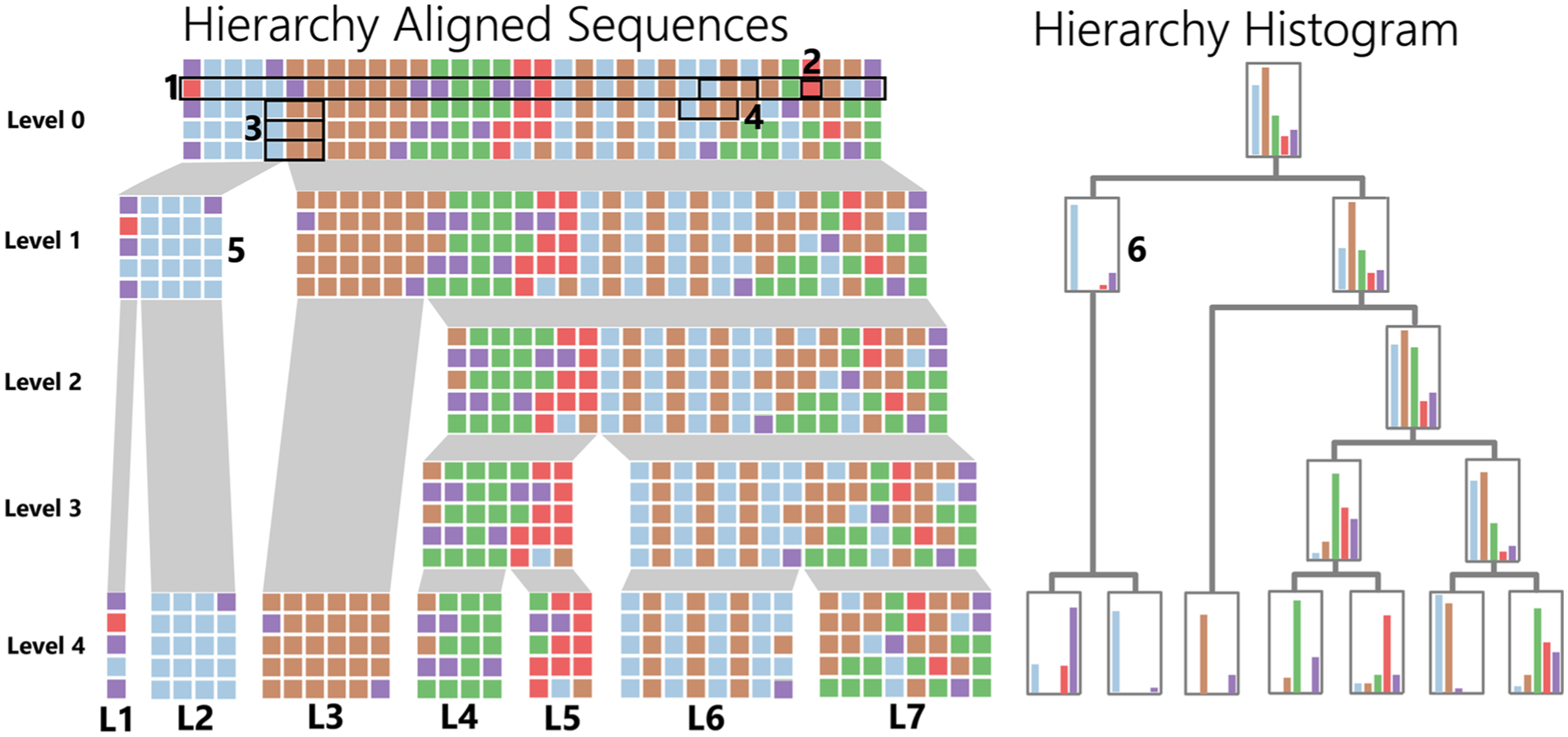
Global staging: On the top left (level 0) are the five original input sequences. A sequence is horizontally displayed (1) with each event (2) in chronological order. Patterns are subsequences present in one or multiple sequences, for example, the blue-brown-brown pattern (3–4). During global splitting these sequences are recursively split in two children represented by the hierarchical flow. For example, the original sequences (top on the left) are split into two children, for example, the left child (5). These children are split again etc. The final children (leaves) are the global stages (L1–L7). This splitting is hierarchical. To determine the splits, the (sub)sequences involved in the split are transformed to a data structure of histograms of their event or pattern frequencies. In this case, the event frequencies are seen on the right. For example, parent 5 on the left corresponds to histogram 6 on the right.

Discovering stages

We believe that four key concepts, related to stage discovery in long sequences, are crucial and differentiate LoLo from related work; hierarchy (T5), explainability (T2–T5), similarity (T3), and interactively redefining stages (T1). We demonstrate how these play a role while presenting our method. We first apply a global splitting, by segmenting the sequences in stages, where the position of the split is the same for all sequences (a “straight” vertical split), see Figure 1. This process is then repeated on the resulting stages to retrieve hierarchical stages, enabling analyzing the stages from different levels of detail. Next, we refine the global split of the final stages to take local deviations into account, called local splitting, see Figure 2. To define a split, we identify groups of subsequences that are behaving similarly (either based on event labels or patterns). For this, a distance measure is needed that defines similarity. We use the distribution of events or patterns within a group of subsequences to describe its behavior, similar to other methods, for example, Otsu’s method.²⁶ The distribution naturally translates to histogram representations, which ease understanding and interpretation, making them suitable for explainability. Additionally, they scale well to long sequences and enable computational similarity, they are used as distance metric between distributions. In general, the distance measure and split condition can be adapted to the application domain. In the next sections, we describe in detail how we build histograms, derive distance functions, and integrate these for global and local staging of long sequences.

Figure 2.

After the global splitting, the leaves (L1–L7, see Figure 1) are used in the local splitting. Each two consecutive leaves are merged, for example, L6 and L7. The subsequences are clustered and per cluster the splitting is run again. This results in the final stages. The local splitting is only done with the leaves of the global splitting. The results from this are used to create the final hierarchy.

Building histograms

As we aim for stages with similar behavior, the discovery depends on both the homogeneous event labels and their order. We assume patterns are precomputed with, for example, the VMSP algorithm^27,28 that provides a concise representation of all patterns.²⁹ The focus of this paper is not on pattern computations. Any pattern algorithm can be used to generate the pattern file. This pattern file, similar to the aligned sequences, is an input file of LoLo. To represent the event data, the (sub)sequences are converted to histograms displaying the event label, for example, histograms in Figure 1 right or Figure 3 top, or the pattern frequency, see histograms Figure 3 bottom. Each bar in the histogram represents the frequency of one unique event label or unique pattern. Visually, the order of the bars is the same for all histograms, alphabetical. Computationally, the order does not matter for the splitting and events or patterns with a frequency of zero are not taken into account. Both discover different stages with other characteristics. For example, when using event labels for splitting, the blue subsequences at the end of every sequence are discovered as a stage, see Figure 3 top. We use patterns of consecutive events to represent often occurring event orders. These generate different stages, see Figure 3 bottom.

Figure 3.

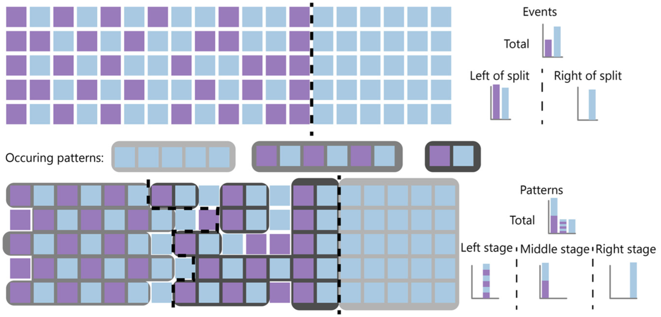
Example of the differences between splitting based on events (top) and patterns (bottom) for the same sequences. There are five sequences with two possible event labels, purple and blue. Assume three possible patterns occur. The background colors indicate where these patterns occur in the bottom sequences. The dotted lines indicate the splits based on events or patterns. The right side indicates the histograms associated with the splits. For explanation purposes, we assume each sequence is their own cluster in the local staging.

Distance measure

The distance measure is based on our definition of a stage. As we want our stages (distributions of events or patterns) to be as homogeneous as possible, we select Information Gain³⁰ to compute the split scores for the staging based on the histograms. Information Gain, often associated with decision trees, aims to split attributes (sequences in our case) such that resulting subgroups are homogeneous:

$E = - \sum_{i = 1}^{n} p_{i} lo g_{2} (p_{i}),$ (1)

where $E$ is the entropy, representing the impurity of a (parent) stage. $p_{i}$ is the probability of randomly selecting an event label or pattern $i$ from the sequences out of all occurring event labels or patterns, $n$ . The probability $p_{i}$ is reflected in the histograms. Next, entropy is used to compute Information Gain, $IG$ :

$\begin{matrix} \begin{matrix} IG = E_{t} - (\frac{e_{l}}{e_{t}} \cdot E_{l} + \frac{e_{r}}{e_{t}} \cdot E_{r}), \end{matrix} \end{matrix}$ (2)

where $E_{t}$ , $E_{l}$ , and $E_{r}$ are the entropy of the sequences before, left of, or right of the split. $e_{l}$ , $e_{r}$ , and $e_{t}$ are the histogram frequencies left, right, and total. The higher the Information Gain, the more entropy is removed and the better the split (in accordance with our definition of a stage).

Global staging

Since we assume sequence alignment and that sequences have the same high-level structure, we deduce the following. The same event labels of the sequences are predominantly grouped around the same indices, for example, the first event of each sequence is at index zero, the second event at index one, etc. LoLo uses an exhaustive greedy search to discover the global splits. This global staging is similar to data reduction strategies as proposed by Du et al.,¹⁸ that is, merging events by time window and merging events into one abstraction. We adapt this by considering time-varying windows and abstract multiple events of multiple sequences in one stage.

First, LoLo determines all potential split indices; index $i$ is a potential split if $i \geq m$ and $i \leq l_{seq} - m$ , where $m$ is the (user defined) minimum number of events per sequence in a stage, and $l_{seq}$ the sequence length. Depending on the sequence length, $m$ should be set large enough to find interesting relations. Second, for each potential split index, LoLo uses the histograms either based on events or patterns, see “Building histograms” subsection, of the subsequences on left and right sides of a potential split. Then, the split score for that index is computed with Information Gain,³⁰ see “Distance measure” subsection. As can be seen in Figure 4, using histograms based on event labels separate, for example, the blue and brown events in stages S1 and S2, see Figure 4. Third, it selects the split with the highest IG and then recursively iterates over the result, to create the desired hierarchy, see Figure 1. The newly added IG is expressed as a percentage compared to the cumulative IG of all its (grand) parent splits. If it is below a user defined threshold the staging stops. We set the default stop criteria to a threshold of 5% because we want to stop splitting before the cumulative IG curve converges. We considered using a maximum number of stages instead, but users typically do not know the desired number of stages. Furthermore, we chose to split a stage into two child-stages for simplicity and interpretability. The resulting stages are grouped hierarchically, see Figure 1 right, to support retrieving detailed information on different levels (T5). See Supplemental material for the algorithm details. Theoretically, the running time is similar to that of a decision tree construction process, $nmlog (n)$ , where $n$ is the sequence length and $m$ is the number of sequences. This is under the assumption that there are not many, that is, tens or more, different event types, otherwise running time increases, see Supplemental material. This splitting, facilitates the use of domain knowledge by iteratively refining stages (T1).

Figure 4.

The final hierarchy after the global and local splitting, see Figures 1 and 2, is displayed on the left. This hierarchy is transformed in a stage hierarchy plot (right). Also, each stage/leave S0–S6 is plotted in the stage similarity plot.

Local staging

LoLo computes local stages as variations of the global stages, which capture local nuances in the global splits using clustering on each two consecutive stages (leaves of the hierarchy). We first cluster the sequences in every two consecutive stages using density-based clustering (DBSCAN),³¹ see Figure 2. We opted for density-based clustering as it does not require to specify the number of clusters. Distances between sequences are computed based on the histograms using the Jensen-Shannon distance.³² We use this distance because we do not want to segment sequences in two homogeneous children, but rather base it on their similarity. We also experimented with dynamic time warping.³³ But this is computationally expensive, even with the relatively short (a couple of hundred or a thousand events) sequences. The density-based clustering method has an epsilon parameter related to what is considered dense and a minimal number of points within that epsilon radius parameter. Second, LoLo computes a new split for each cluster or noise sequence based on the histograms. The splitting is performed similar to the global splitting. Now, LoLo only considers the information of the two consecutive stages of that cluster or noise sequence, see Figure 2. Based on this, the final hierarchy is seen in Figure 4. There is a (user defined) maximum allowed deviation to avoid large deviations from the global split. This results in the local stages, see Supplemental material for details. We use an epsilon 0.2 and a minimal number of points of 2 for the density-based clustering, which were experimentally found adequate for our data.

Visualization

In this section, we describe the visualization part of the LoLo method based on its four key concepts; hierarchy, explainability, similarity, and interactively refine stages. For an overview of the interactions, see Supplemental Video, and for the code see https://github.com/SannevdLinden/Long-and-a-Lot.

Hierarchy

For the stage hierarchy plot, see Figure 4, users should be able to inspect different (aggregated) levels of detail (T5) (two examples of the hierarchy plot are Figure 5(c1) and (c2), compare them (T3), and understand transitions (T4). As mentioned in the Global Staging, LoLo discovers stages with a top-down hierarchical approach implementing a user-based focus and context approach enabling scalability and flexible switching. The stages are the leaves of the hierarchy. The top part of the stage hierarchy plot represents the hierarchy levels, see Figures 5(d) and 6. LoLo represents each level of this hierarchy using an adapted icicle plot. Each stage has a header label with the stage name, for example, S0, see Figure 5e. This hierarchy visualization provides users insights into how the data is split into stages and offers different levels of detail (T5).

Figure 5.

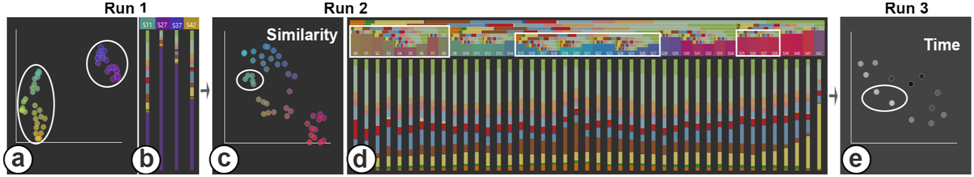
LoLo’s interface where each stage is represented as a circle in the stage similarity plot (b). Stages are displayed in an icicle plot with different levels of detail (c1, c2), and hierarchy on top (d); the stage header color (e) corresponds to the scatterplot (b) colors to identify similar stages. The horizontal stacked bar charts (d) represent the frequency of each event label for each level of the hierarchy (e.g., the ascendants of the stages) and are colored based on the event label. Examples of user-selected (a) display levels are: the aggregated level with and without (c1) normalization of the bar charts, and the detailed level (c2). Normally, only one display level, for example, c1 or c2 is displayed. The bars of the histograms in c1 and d, and the events in c2 are colored based on event labels.

We use an adapted icicle plot because it preserves the temporal order of the stages, allows to show abstracted information of each stage hierarchically, and provides the ability to focus on stages of interest without loosing the hierarchical overview. Initially, the whole hierarchy of stages is displayed, providing a high-level overview for each stage in the hierarchy. Horizontally stacked bar charts, see Figure 5(d), represent the proportion of the different event labels or patterns (depending on the global staging distance measure) that occur in each level of the hierarchy for all ancestors of the stages. If there is insufficient space to display the stacked bar chart, the top frequent labels or patterns are displayed depending on the available space. Also, a red triangle is added in the lower right corner to indicate that some label or pattern frequencies are left out of the visualization. LoLo enables users to close (collapse) and open (expand) stages, see Figure 6. This provides users with a focus and context mechanism. The context switching by changing levels is animated to preserve users’ mental model. All expanded stages, receive the same amount of screen space to emphasize that each stage is potentially equally important. LoLo enables users to expand ancestors of the stages, see Figure 6(b). A parent is displayed in the same way as a child stage, with the collapsed children displayed underneath, see Figure 6(b1). The content of the expanded stages and (grand)parent stages are horizontally aligned to make comparison (T3) easier. Overall, we adapted an icicle plot to be able to display the hierarchy of stages in relation to the sequence data both chronologically and hierarchically. Through different representations, for example, the stacked bar charts and opening or collapsing stages, we provide further information for the understanding of the method.

Figure 6.

Example of the hierarchy where the (grand)parent stages are indicated in purple and blue, respectively; (a) describes what happens if users close the redly marked stages by clicking, (b) describes what happens if users expand a parent or grandparent, indicated in green. Their children are closed (b1).

Explainability

Understanding the constructed stages and their transitions (T4) is important because there is no way to validate the stages automatically. LoLo displays the subsequences in an expanded stage on three different aggregation levels; as a most aggregatedoverview the corresponding histograms of the expanded stages are shown (1), see Figure 5(c1); as compressed information (mid-level) where each × consecutive events of the subsequences are merged into one event (2); or as detailed information (3), see the rectangles representing individual events, such as the blue ones in Figure 5(f). By default, LoLo displays the most aggregated overview of all the discovered stages. The aggregated overview consists of histograms because these are easy to interpret and scalable visualizations that increase the understandability. When users hover over a stage header, LoLo shows a tooltip with the time of the earliest and latest events. Users can choose between non-normalized and normalized bar charts. Non-normalized bar charts inform users about the number of events or patterns, depending on the global staging distance measure. Normalized bar charts help to compare the event label or pattern frequency histograms, depending on the global staging distance measure, to understand the computed splits. This increases explainability because the splits are based on differences between those histograms. For the normalized bar chart, the highest frequency in that chart is scaled to a hundred percent and the other bars are scaled relative to this. To increase visual scalability, the histograms can be shown in different levels of detail depending on the screen space; vertical stacked bar charts, see Figure 10(d), and histograms with, see Figure 5(c1), and without axis, see Figure 8(b). For patterns, the bar representing it is colored based on the pattern, see Figure 11. For example, if a pattern consists of event A followed by event B, the first half of the bar representing this pattern is colored with the label A color and the second half with the label B color. If there are more than 20 unique patterns, the 20 most frequent ones are included in the bar charts for visual scalability reasons.

The detailed information view displays the original subsequences present in the stage to verify in which (groups of) sequences certain event labels or patterns occur that are responsible for the stage splits. Each ordered subsequence is represented by horizontally aligned event blocks. The different stages’ subsequences are horizontally aligned to enable visual comparison. The color of an event block is determined by its label. The event types scale visually to the 15 labels with the highest frequency, based on the qualitative scales from ColorBrewer.³⁴ This ensures the colors of the different events are still distinguishable. All other label categories are colored gray. This means that in LoLo the components seen in Figure 5(c1), (c2), and (d) are colored using this color scheme. The mid-level displays a compression of the events to increase visual scalability. For example, if there is screenspace for 10 events and a hundred events present, each of the 10 events is compressed into one based on the highest occurrence frequency. By zooming in and out, this compression ratio becomes less or more. This relates to the bucketing events using a fixed time window data reduction strategy.¹⁸ To help with verification, users highlight event labels and patterns interactively. At the compressed or detailed level users identify why certain stages were discovered and how they differ (T2, T3, T5). Users can manually select and highlight patterns at the compressed or detailed level.

Users can cluster the subsequences within one stage for visual inspection based on their event labels. Users are free to change the epsilon value, related to what is considered dense, for density-based clustering of these subsequences. This epsilon is for clustering within one stage, not the epsilon for clustering in the local staging between consecutive stages. A consequence of the clustering is that the horizontal alignment of sequences, the subsequences of sequence × have the same vertical position in all expanded stages, over the different stages is no longer preserved. Due to clustering, this vertical position differs per stage, but via highlighting interaction, the subsequences of the same sequence are identified. To further ease comparison (T3), LoLo enables users to align the sequences horizontally based on the clustering of a selected stage, see Figure 9. The clusters of the detailed level and mid-level are the same and based on the detailed sequence information. Gray arrows will appear on the sides to indicate when more sequence information is available through panning to the left or right within one stage. To aid the comparison (T3), we implemented linked zooming and panning to ensure that the horizontal alignment of the bar charts or the blocks are synchronized.

Stage similarity

The stage similarity plot, see Figures 4 and 5(b), and the stage headers in the hierarchical plot, see Figure 5(d) and (e), enable users to identify stage similarities dependent and independent of time (T2). Each stage (leaves of the hierarchy) is represented as a circle in the stage similarity plot, see Figure 5(b). We use UMAP³⁵ for this stage analysis, where pairwise distances are computed using the distance metric as selected for the global splitting, see “Distance measure” section. The circles are semi-transparent to indicate density. Users typically need to identify how and when stages transition over time (T4). Therefore, by default, the headers of the stages and circles in the similarity plot are colored in grayscale based on their timestamps to identify the re-occurrences over time in the similarity plot. Another option is to project a 2D colormap on top of the scatterplot, where the four corner colors originate from Steiger et al.³⁶ Users are enabled to color the circles and stage headers based on the 2D colormap, see Figure 5 (T2). This means that in LoLo the components seen in Figure 5(b) and (e) are colored using this color scheme. (Grand)parent headers are colored the same as the header color of their middle leave. An example of two similar stages are stage S0 and S7 in Figure 5. The headers both have a yellow-green color, for example, the header of S0 (Figure 5(e)). The S0 bar chart describes this stage as many blue events, some purple events, and little red events. S7, see Figure 5(f), also has the same composition of event labels. There are several interactions available to users. When users hover over a circle, the corresponding stage is highlighted in the stage hierarchy plot. By selecting multiple circles, the stages represented by these circles in the stage hierarchy plot are expanded. When users click on a circle, the stage in the stage hierarchy plot collapses or expands, depending on its state. The circle size depends on the stage state, that is, large if expanded, small if collapsed.

Interactively redefining stages

Based on the hypotheses of the users, different aspects of the data are of importance. Therefore, users are enabled to redefine the stages (T1) by adapting the parameters, see Use Scenario Neighborhood Complaints Data for an example. The different parameters are the stop condition for the splitting (cumulative IG percentage), the maximum event deviation between a local and global split, the minimum number of events per stage, and whether event or pattern frequency histograms are used for the global and local staging. Filtered-out sequences and event labels will disappear from the visualization. When stages are based on events, the filtered-out event labels are not taken into account during staging recomputations. On the detail level, events having a filtered-out label are replaced with an empty space to preserve the multiple sequence alignment. The redefinitions are interactive due to the choices made on the algorithm used to build the hierarchy. The methods have relatively low computational costs while being informative.

Evaluation

We first evaluate the interactivity of LoLo by analyzing the staging algorithm’s running time. Second, we compare LoLo against a baseline of fixed staging. Third, we evaluate LoLo with two use cases on two real-world data sets.

Computational

We claim that LoLo can be used interactively to refine the stages. Here we discuss and evaluate the running time for computing the stages. We use the electrical energy consumption data from 37 different buildings at our university campus from 2019 up to 2022. The data is provided as a time series; to transform those into events, we bin the data in six categories/labels from low to high using quantiles normalized per building. Each sequence represents 1 year of data for one building and each event the binned energy usage of a certain point in time. We align the data based on their timestamps. Only 0.5% of all the events are gaps introduced by the alignment due to missing data and leap year. There are 152 sequences, each with a length of 35,136 events. These precomputations generate the input file for LoLo.

The global staging depends on the number of splits, which relates to the depth of the hierarchy and the stage parameter, responsible for the number of stages. The local staging depends on the number of splits, which relates to the number of clusters and the staging epsilon parameter. To provide an indication of the running times, see Figure 7 and Supplemental Material. The experiments were run on a conventional laptop (Intel i7-9750H CPU, 32GB RAM). Considering a sequence length of approximately 35,000 events and the assumption that users recompute the staging, but not extremely frequently during one use, we consider this running time of approximately 13 and 37 s for staging based on events or patterns, respectively, adequately for supporting the analytical and exploration workflow. Increasing the event types, that is, the number of quantiles in the energy data set, for example, to a hundred event types, increases the running time for staging based on events. However, increasing the staging epsilon reduces the total running time and the number of splits. Also, more event types in this dataset mean fewer patterns. Moreover, increasing the number of sequences increases the running time. When the number of sequences increases, relatively less time goes to the splitting and more to the other functions in the staging algorithm. 84% and 91% of the staging time goes to splitting based on events and patterns, respectively, for 10 sequences, and 32% and 9% of the staging time goes to splitting based on events and patterns, respectively, for a thousand sequences. See Supplemental Material for the details. Overall, the running time for computing the stages of long sequences based on events is adequately for supporting the workflow but increases when the number of event types or sequences grow.

Figure 7.

Staging computation times (left) and number of splits (right) for LoLo’s staging algorithm for sequences of different lengths, based on splitting on events and patterns. The percentage indicates how much of the sequence length of the energy data from the energy use case is included. For example, 50% are the first 6 months of all the sequences. The stage, minimum event, maximum deviation, and staging epsilon parameters are 0.025, 500, 100, and 0.2, respectively. In total, there are 100 unique patterns and 378,124, 284,705, 186,050, and 92,366 patterns in the 100%, 75%, 50%, and 25%, respectively.

Baseline comparison

We compare LoLo’s staging method to a baseline method where we use fixed time-windows. Comparing LoLo to dynamic staging baselines is hard, because there is no defined baseline neither is there a ground truth. Moreover, if we would select a method, such as from Guo et al.,⁸ this likely results in different stages compared to our method, but we cannot conclude one is better over the other as there is no ground truth. We included energy data for the month of January of 1 year. This results in 38 sequences of length 2976 events. We used two different time windows for the fixed staging; either 1 week or 1 day. Figure 8(a) shows that fixed staging of 1 week gives three very similar stages (second to fourth bar chart) since the weekly pattern is similar. Fixed staging per day gives many stages, we can recognize the weekend days, see circles in Figure 8(b). It is hard to get an overview of the similarity between stages and where they repeat over time. Moreover, similar semantic consecutive stages could be merged. As Figure 8(c) shows, our staging based on events is, overall, able to differentiate between holiday, weekends and weekdays based on the content of the stages. The stage header colors show where similar stages are repeated and similar workdays are merged together in one stage. Friday nights and Monday mornings are, in general, included in the weekends as well since people are not working yet and there is low energy usage. This separation is not present in the fixed staging. In Figure 8(d); splitting based on patterns, the staging has trouble separating Mondays and Fridays from the weekend and the work weeks often consist of multiple consecutive stages, but working periods are also visible. There are also multiple occasions in which there is no trivial or meaningful definition of a fixed window, for example, the hospital example from the Introduction. It could take several refinements and re-computations of the stages to find the suitable stages for a data set, since the number of stages is unknown upfront. Therefore, the flexibility to refine the stages interactively is important (T1).

Figure 8.

Fixed staging based on weeks (a) or days (b) compared to our staging based on events (c) or patterns (d). White circles indicate weekends in b and work periods in (d). The yellow stages are work periods in (c). An example stage histogram of working and weekend periods is displayed in (c) and (d).

Use case energy consumption data

We evaluated LoLo with two users: P1, a data scientist in the energy sector, and P2, a data scientist researcher mainly working with genomics data. The goal is to discover high-level structures in the energy usage of buildings and similar and outlying energy usage periods over the year. P1’s evaluation is leading in this section. P2’s feedback is mainly used from a usability point of view because P2 is familiar with sequence data but in a different domain. Based on the same set of specific tasks, see below, and our instructions, we let P1 and P2 interact with LoLo. Afterward, they filled in a five-point Likert scale system usability scale³⁷ questionnaire, where a score of one is strongly disagree and a score of five is strongly agree.

We initialized LoLo based on event staging (using events for global and local splitting, stage parameter of 0.025, minimum events 500, and maximum deviation 100) and color the stage headers based on similarity. 25 stages are discovered, S0–S24. We asked the participant to share their first impression of the yearly energy data in the high-level overview. The first thing P1 noticed is that the winter (at the beginning, until March, and end of the year, November/December) and summer (the other parts of the year) periods differ (T3). Also, the first and last stages correspond with the Christmas holiday and are more similar to the summer period, likely because the buildings are closed (T2). Furthermore, there is one stage, S6, with a header color different from the surrounding winter stages, which P1 also suspected as a holiday period (T2). However, it is not a holiday period and something else is going on, see below.

Two main clusters are visualized in the stage similarity plot. Next, we asked the participant to select multiple points in the stage similarity plot from each cluster to identify the differences between the clusters, see Figure 9(b). All the stages that were not selected in the scatterplot are closed, such that only the selected stages remained expanded. After selecting two stages from each cluster, P1 and P2 noticed that the high-level histograms of the different clusters almost have an inverse relation of ascending or descending occurrence frequency from q1 to q6 (T3). Since the histograms directly relate to how the stages are split and the hierarchy is build, they help users reason about why these stages exist. This is harder to do with state-of-the-art methods where stage summaries are not related to the splitting of the stages, for example, Guo et al.⁸ We also asked the participant to make this comparison on the low and mid-level (T5) by changing these four expanded stages from a high-, to a low-, and mid-level. The low level is too detailed, according to P1, to conclude something about the clusters quickly. P1 noticed on the mid-level that blue stages have indeed more events of darker colors and that there is probably some night and day rhythm within the stages.

Figure 9.

Three expanded stages on the mid-level describing the Christmas transition, S22–S24 (from the 10th of December to the 31st) see (a), where the sequences are ordered based on the clustering, see C1–C6, of stage S24. For example, if sequence 10 is displayed (vertical position on the screen) as the third sequence from the top in S24, then the subsequences of sequence 10 in S22 and S23 have this same vertical position, that is, third from the top in S22 and S23. The event labels are q1 to q6, low to high energy, and dark green to light green (see Menu). Most buildings, see C1 and C3, have many high-energy events in the winter (S22, the pink stage header), fewer high-energy events towards the Christmas break (S23), and even less during the Christmas break (S24). While some buildings have many high-energy events in all three stages, see C2. (b) describes the two clusters of all the 25 stages (a + d): blue and pink. (d) describe the collapsed stages S0–S21. One anomalous stage (S6) is surrounded in time by pink stages (S5, S7).

Afterward, we asked the participant to select the last three stages to investigate the transition to the Christmas holiday. Now, only the last three stages are expanded and the rest is closed. Based on the mid-level, P1 mentioned that there is a daily pattern, see Figure 9, and that some buildings are more similar to each other. We asked P1 to select the clustering option and align them based on the clustering of the last stage to more easily compare (T3) sequences within stages and their transition (T4), see Figure 9. P1 noticed that some buildings in S24 only have the lowest energy level. Also, P1 mentioned that there is still higher energy usage in C2 and C4. C2 does not have a daily pattern and is always high. P1 wondered if machines are running constantly or if something else is happening. Moreover, P1 observed that darker sequences in S24, for example in C1, have higher energy usage, probably during the day, before Christmas. Similar, P2 mentioned that the light events followed by dark events pattern from the previous stages disappears in S24 for C1 and C3. Multiple levels of detail, among which the mid-level, contribute to the understanding of the stages and help compare them.

We asked P1 to investigate the outlying stage S6 (T2), see Figure 9(b), based on the high-level bar charts by expanding S6 and the surrounding stages and closing the others. S6 is a blue colored stage surrounded by pink colored stages, based on the stage headers. P1 noticed that there is missing data (gaps) by the frequency of the gap category in the high-level histogram. This is similar to the data in December, but otherwise, there is not much difference to S7. We explained that we can confirm if that stage was formed due to the gaps by rerunning (T1) the staging without gaps. After rerunning the stages, P1 saw, that the time period of the previous S6 is now similar to other winter weeks in the high-level overview. This was also noticed by P2. This is an example of how we think that LoLo interactively helps to redefine the stages based on the explanation of the stages. Based on the histograms, which explain that there are many gaps but no other large differences compared to surrounding stages, users insert this knowledge into the recomputation and get stages that better reflect the data. This redefining of the stages of long sequences is hard with other methods from related work.

We also wanted to know if the patterns present a different data perspective. Therefore, we instructed P1 to select the pattern buttons and interactively switch to frequent patterns (T1) for the global and local splitting. P1 mainly noticed at the high-level that the first week of January is not the same as the summer period and last stage anymore. We asked P1 to select several stages to keep expanded and close the rest to identify their differences. By selecting the first and the last stage together with a second stage similar to S0 and a winter stage before the Christmas holiday, P1 compared the high-level bar charts. P1 mentioned that S0 and a similar stage, according to their stage header color, have many patterns that consist of many light-colored events after each other or patterns consisting of only dark-colored events; not many mixed patterns. P1 noticed that the winter stage mainly has light-colored patterns, and the last stage mainly has dark-colored patterns. Indicating that LoLo helps to explain the role of the patterns in the discovered stages.

Overall, P1, who is experienced with events and visualizations,found it relatively easy to use LoLo, scoring a five for ease of use and confidence, and a one for needing to learn a lot of things, see Supplemental material for all scores. P1 mentioned that this is a system for people with knowledge about data analysis, and even within that group, most will need a mini-course to learn it. P1 gave a score of three for learning this system quickly. P2 had more trouble interacting with LoLo and found it difficult. P2 gave a 3.5 for unnecessary complexity because P2 forgot which options existed and had trouble knowing what to do and when in this short usage period. Therefore, P2 gave a score of two for confidence and that people would learn it quickly. Also, P2 thought she needed to learn a lot to use LoLo, a score of four. Although, P2 still gave a four for easy to use. Also, P1 mentioned that some interactions could be improved and, therefore, gave a score of three for inconsistency in the system. P2 also mentioned that selecting stages is not so easy. Moreover, P1 gave a score of three for using the system frequently. P1 explained that LoLo possibly helps to give P1 insights, but if P1 wants to communicate this to partners and clients, which often happens, then P1 needs to translate the information into simpler plots. This was the biggest drawback of LoLo, according to P1. On the other hand, P1 liked the different levels of detail and the ability to rerun the data the most based on this short usage. P2 also liked the switching between different detail levels.

Use scenario neighborhood complaints data

We describe a usage scenario using complaints data from five neighborhoods in the city of Eindhoven.⁷ We carry out this scenario, no users were involved. We want to discover high-level complaints patterns, when they occur, and if they reoccur over the year. A sequence is 1 year of data from one neighborhood and each neighborhood has 11 years of data. An event is a complaint. We have 55 sequences, each of length 8980 events. We aligned the data based on their timestamps: the first event of each week is aligned because we expect that time of year influences the occurring events. This results in 57% of the events being gaps. The events are categorical and have 15 possible main categories (including gaps). We gave the main categories an English name, for example, greenery or animal, representing the names of all its subcategories.

We initialize LoLo with the defaults; a stage parameter of 0.05, 100 minimum events, and 50 maximum deviation. Initially, we see two clusters, see Figure 10(a) white circles. After inspecting the normalized histograms of stages of each cluster, it is hard to identify the differences (T3) between the stages except for the gaps, see purple bars Figure 10(b). The proportion of these purple bars differs between the two clusters, but the other colors are hard to compare. Therefore, we rerun LoLo without the gaps (T1) because we want to know the high-level structure based on the event labels rather than being dominated by the gaps, see Figure 10(c) and (d). Now, several stage clusters (T2) and their transitions (T4) appear in the stage similarity plot, see Figure 10(c) white circle for an example cluster. Looking at the colors of the stage headers based on similarity, we see that there is a gradual yearly transition, Figure 10(d). The color of the headers changes from orange to blue to pink. Also, we run the staging again (T1) with a stage parameter of 0.1 because there are quite some similar stages with the same (grand)parent and similar header colors after each other, see the white boxes in Figure 10(d) white boxes. This is an indication that there might be too many stages. By changing the stage parameter to 0.1, the stages are merged into fewer stages. In the stage similarity plot, we can see that, for example, the last two stages, representing the last days of the year, start to transition from the previous stages, see Figure 10(e) white circle. In order to easily see this, the stage headers are colored in grayscale based on their temporal order. In this manner, LoLo helps us to interactively redefine the stages based on the stage explanations, that is, stacked bar charts, stage similarity, that is, header colors, and hierarchy.

Figure 10.

Snippets of LoLo with complaints data. With 50 stages (a), there are two clusters, that appear to differ mostly on the gaps (purple part of the bars), see (b). By rerunning LoLo such that it excludes gaps (resulting in 43 stages), we see less separated clusters as well as some transition clusters (white circle in (c)). A yearly pattern in the stage headers (d) is visible now. There are similar stages after each other that share a (grand)parent (white boxes in (d)). Reducing the Information Gain parameter further (another rerun of LoLo), results in 13 stages (e). Stages are colored by temporal order (dark to light gray) and the white circle is indicating the last two stages.

To identify the differences and similarities (T2) between the stages we used the normalized high-level bar charts, we filtered out categories that only contribute a small percentage to all the events and/or that stay approximately constant throughout the year. For example, during the summer period, that is, mid-May to the end of August, there are relatively more greenery and less lighting events than the rest of the year.

To find out more about the event order of the stages, we rerun the staging with the patterns for the global and local splitting (T1) and a stage parameter of 0.3. We see that one stage, S5, has by far more patterns than the other stages, mid of April until end of August. We see this by using the non-normalized high-level bar charts and looking at their height. To see the stage differences (T3), we look at their normalized high-level bar charts, see Figure 11. For example, the large stage has relatively many patterns with greenery events, brown, combined with animal, orange, see Figure 11 white rectangle. Although, the differences are not directly obvious, maybe because the unique patterns do not occur often in the entire data set; frequency is maximum 182. This explains why these stages are discovered.

Figure 11.

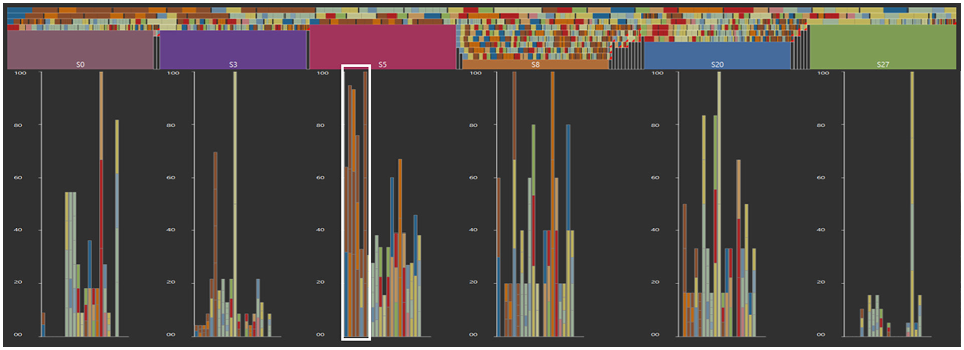
Normalized high-level from the complaints data, where the staging is based on patterns. Each bar represents a pattern, the color in the bar represents the events in the pattern from bottom to top. S5 has relatively many patterns containing greenery events, brown events, see the white box.

Discussion and conclusion

This paper presents LoLo, a novel visual analytics approach to discover, explore, and analyze high-level structures in long event sequences by discovering stages. These stages are of flexible time windows because they are created based on their content. These stages have four key concepts making them novel; they are hierarchical and explainable, their similarities are computed and interactive refinement is possible. Users are enabled to interactively refine stages by rerunning LoLo with different settings (T1) to highlight different aspects of the data that describe the high-level structure of the sequences. Together with the stage similarities, and hierarchy, LoLo enables users to identify meaningful stages (T2) and compare (T3) them and their transitions (T4) on different levels of detail (T5). Two real-world use cases show that LoLo enables us to find high-level structures in long sequence data which would not be achievable with staging using fixed window lengths. Experiments show that users can indeed rerun the staging interactively. Moreover, the use cases show that LoLo enables users to analyze long event sequences of lengths of around 35,000 events.

LoLo is not domain dependent. However, the similarities that define the stages might need to be adapted to specific domains. LoLo needs event sequence data that progresses as input. Otherwise, there is no high-level structure. Moreover, there are several considerations. We considered combining the event label and pattern splits, however, if we have a proposed split based on the event labels and the patterns, it is unclear how to combine these. We cannot just take the highest split score because their split scores represent different aspects. Also, it is unclear which event split to match with which pattern split. Therefore, users either determine the global stages on the event label or the pattern histograms, and can easily switch between the two. We also considered clustering sequences before any global splits are made, so the staging could be computed per cluster to optimize for homogeneous stages. However, for this a distance metric between sequences is needed, this is different from the IG distance metric to split sequences. The Levenshtein distance³⁸ is the most common distance measure to compute distances between two sequences. However, for long sequences, many insertions, deletions, and replacements are needed. After normalization, distances are too similar, resulting in a hierarchy where often only one sequence is added to the main cluster at each step.³⁹ Moreover, the computation time does not allow for interactivity. To the best of our knowledge, no other distance metric for sequences mitigates these shortcomings. We leave this for future work.

Also, LoLo currently cannot detect certain data constructs, such as concurrency or parallelism, between the different stages. By providing stages with summaries, the cognitive load is reduced because users get an overview and for selected stages of interest users get more detail. The adapted Icicle plot keeps the time-aspect of the stages and the hierarchy with the different levels of detail help to navigate to interesting data subsets while keeping track of the overall context. However, the horizontally stacked bar charts encoded in the hierarchy, see Figure 5(d), could be improved because this part looks busy. Different aggregation schemes, for example, visualizing the majority event, may offer solutions. Moreover, if sequences do not fit the screen-space vertically, users have to pan or zoom out to get all the sequences on the screen, which increases the cognitive load. By also compressing the sequence vertically, perhaps in a similar visual manner as Sequen-C,³ LoLo could visually support scalability in the amount of sequences. These cognitive load reducing summaries could also omit potentially interesting relations. We currently use a simple aggregation scheme for the mid-level. Different aggregation schemes, such as mentioned in Sequence Surveyor,⁴⁰ could also be added. Furthermore, the parameter setting is influenced by the specific data characteristics and need to be tuned to get optimal results. Finding this optimum might not be trivial. However, it can be found through iterative interactive exploration.

There are several opportunities for future work. For example, a more formal, extensive user study will provide more insight to improve and validate LoLo. Also, it would be interesting to have additional interactions in the staging to, for example, redefine the stages arbitrarily. However, this would need quite some effort to coordinate with the stage generation. Additional interactions to promote comparison could be added as well, where users are able to extract and rearrange stages. A next logical step is to extend LoLo to multivariate sequence data, where the multivariate attributes are incorporated in the staging. Furthermore, the results are as good as the distance metric is able to capture the relevant information. Further research to alternatives would be useful, for example, Jaro-Winkler distance.⁴¹ It would be interesting to improve computational times for, for example, the staging, as evaluated in “Computational” subsection, or the drawing of the elements on the screen. The field of progressive VA might provide inspiration. Moreover, the colors can be improved. Currently, the categorical colorscheme and the colormap make LoLo colorful with possibly similar colors, for example, both colorschemes have a shade of purple. All in all, LoLo enables users to identify insights in long sequences with a lot of events. LoLo helps potential users to identify the high-level structure in long event sequences by enabling them to interactively redefine hierarchically discovered stages which is superior to baseline fixed window stages or not understandable dynamic stages. Users have the ability to explore multiple aggregation levels for comparison between stages and within one stage. Through this method we aim to provide users with new perspectives on long event sequence data.

Supplemental Material

sj-pdf-1-ivi-10.1177_14738716251372584 – Supplemental material for Long sequences with a lot of events (LoLo): A visual analytics approach for analyzing long event sequences

Supplemental material, sj-pdf-1-ivi-10.1177_14738716251372584 for Long sequences with a lot of events (LoLo): A visual analytics approach for analyzing long event sequences by Sanne van der Linden, Bram Cappers, Anna Vilanova and Stef van den Elzen in Information Visualization

Footnotes

Acknowledgements

We thank the experts for their feedback. We also thank our university’s real estate department for the usage of the energy data set.

ORCID iDs

Sanne van der Linden

Bram Cappers

Anna Vilanova

Stef van den Elzen

Funding

The authors received no financial support for the research, authorship, and/or publication of this article.

Declaration of conflicting interests

The authors declared no potential conflicts of interest with respect to the research, authorship, and/or publication of this article.

Supplemental material

Supplemental Material for this article is available online.

References

Gotz

Stavropoulos

Decisionflow: visual analytics for high-dimensional temporal event sequence data. IEEE Transactions on Visualization and Computer Graphics 2014; 20(12): 1783–1792.

van der Linden

Wulterkens

van Gilst

, et al. Flexevent: going beyond case-centric exploration and analysis of multivariate event sequences. Computer Graphics Forum 2023; 42: 161–172.

Magallanes

Stone

Morris

, et al. Sequen-c: a multilevel overview of temporal event sequences. IEEE Transactions on Visualization and Computer Graphics 2021; 28(1): 901–911.

van der Linden

de Fouw

van den Elzen

, et al. A survey of visualization techniques for comparing event sequences. Computers & Graphics 2023; 115: 522–542.

Johnson

Bulgarelli

Shen

, et al. Mimic-iv, a freely accessible electronic health record dataset. Scientific Data 2023; 10(1): 1.

Cappers

BCM

Meessen

Etalle

, et al. Eventpad: rapid malware analysis and reverse engineering using visual analytics. In: Staheli

Paul

Kohlhammer

, et al. (eds.) 2018 IEEE Symposium on Visualization for Cyber Security (VizSec). IEEE, 2018, pp.1–8.

Gemeente Eindhoven. Meldingen openbare ruimte, https://data.eindhoven.nl/explore/dataset/meldingen-openbare-ruimte (2023, accessed 14 November 2023).

Guo

Jin

Gotz

, et al. Visual progression analysis of event sequence data. IEEE Transactions on Visualization and Computer Graphics 2018; 25(1): 417–426.

Nusrat

Harbig

Gehlenborg

Tasks, techniques, and tools for genomic data visualization. Computer Graphics Forum 2019; 38: 781–805.

10.

Gotz

. Soft patterns: Moving beyond explicit sequential patterns during visual analysis of longitudinal event datasets. In: Proceedings of the IEEE VIS 2016 Workshop on Temporal & Sequential Event Analysis, IEEE, 2016.

11.

Guo

Zhao

, et al. Eventthread: visual summarization and stage analysis of event sequence data. IEEE Transactions on Visualization and Computer Graphics 2017; 24(1): 56–65.

12.

Wang

Mazor

Harbig

, et al. Threadstates: State-based visual analysis of disease progression. IEEE Transactions on Visualization and Computer Graphics 2021; 28(1): 238–247.

13.

Wang

Zhang

Tang

, et al. Unsupervised clickstream clustering for user behavior analysis. In: Proceedings of the 2016 CHI Conference on Human Factors in Computing Systems. 2016, pp.225–236. New York, NY: Association for Computing Machinery.

14.

Guo

Jin

, et al. Survey on visual analysis of event sequence data. IEEE Transactions on Visualization and Computer Graphics 2021; 28(12): 5091–5112.

15.

Chen

Puri

Yuan

, et al. Stagemap: Extracting and summarizing progression stages in event sequences. In: Abe

Liu

, et al. (eds.) 2018 IEEE International Conference on Big Data (Big Data). IEEE, 2018, pp.975–981.

16.

Cappers

van Wijk

JJ.

Exploring multivariate event sequences using rules, aggregations, and selections. IEEE Transactions on Visualization and Computer Graphics 2017; 24(1): 532–541.

17.

Chen

Ren

Sequence synopsis: Optimize visual summary of temporal event data. IEEE Transactions on Visualization and Computer Graphics 2017; 24(1): 45–55.

18.

Shneiderman

Plaisant

, et al. Coping with volume and variety in temporal event sequences: Strategies for sharpening analytic focus. IEEE transactions on visualization and Computer Graphics 2016; 23(6): 1636–1649.

19.

Chen

Yue

Plantaz

, et al. Viseq: Visual analytics of learning sequence in massive open online courses. IEEE Transactions on Visualization and Computer Graphics 2018; 26(3): 1622–1636.

20.

van den Elzen

Holten

Blaas

, et al. Reducing snapshots to points: a visual analytics approach to dynamic network exploration. IEEE Transactions on Visualization and Computer Graphics 2015; 22(1): 1–10.

21.

Cohen

Grossman

Morabito

, et al. Identification of complex metabolic states in critically injured patients using bioinformatic cluster analysis. Critical Care 2010; 14(1): 1–11.

22.

Yang

McAuley

Leskovec

, et al. Finding progression stages in time-evolving event sequences. In: Proceedings of the 23rd International Conference on World Wide Web, 2014, pp.783–794. New York, NY: Association for Computing Machinery.

23.

Kwon

Anand

Severson

, et al. Dpvis: Visual analytics with hidden markov models for disease progression pathways. IEEE Transactions on Visualization and Computer Graphics 2020; 27(9): 3685–3700.

24.

Zeng

Wang

, et al. Emoco: Visual analysis of emotion coherence in presentation videos. IEEE Transactions on Visualization and Computer Graphics 2019; 26(1): 927–937.

25.

Feng

Doolittle

RF.

Progressive sequence alignment as a prerequisitetto correct phylogenetic trees. Journal of Molecular Evolution 1987; 25: 351–360.

26.

Otsu

A threshold selection method from gray-level histograms. IEEE Transactions on Systems, Man, and Cybernetics 1979; 9(1): 62–66.

27.

Fournier-Viger

Gomariz

, et al. Vmsp: Efficient vertical mining of maximal sequential patterns. In: Advances in Artificial Intelligence: 27th Canadian Conference on Artificial Intelligence, Canadian AI2014, Montréal, QC, Canada, May 6-9, 2014. Proceedings 27. pp.83–94. Springer, Cham.

28.

Fournier-Viger

Lin

JCW

Gomariz

, et al. The spmf open-source data mining library version 2. In: Machine Learning and Knowledge Discovery in Databases: European Conference, ECML PKDD 2016, Riva del Garda, Italy, September 19-23, 2016, Proceedings, Part III 16. pp.36–40. Springer, Cham.

29.

Fournier-Viger

Lin

JCW

Kiran

, et al. A survey of sequential pattern mining. Data Science and Pattern Recognition 2017; 1(1): 54–77.

30.

Witten

Frank

Hall

. Data mining: practical machine learning tools and techniques. A volume in The Morgan Kaufmann series in data management systems, Morgan Kaufmann. 3rd ed. 2011. Morgan Kaufmann Publishers. ISBN 978-0-12-374856-0.

31.

Ester

Kriegel

Sander

, et al. A density-based algorithm for discovering clusters in large spatial databases with noise. In: KDD, volume 96, 1996, pp.226–231. AAAI.

32.

Endres

Schindelin

JE.

A new metric for probability distributions. IEEE Transactions on Information Theory 2003; 49(7): 1858–1860.

33.

Keogh

Ratanamahatana

CA.

Exact indexing of dynamic time warping. Knowledge and Information Systems 2005; 7: 358–386.

34.

Brewer

Harrower

Sheesley

, et al. Colorbrewer 2.0 color advice for cartography, https://colorbrewer2.org/ (2013, accessed 5 October 2023).

35.

McInnes

Healy

Melville

Umap: Uniform manifold approximation and projection for dimension reduction. arXiv preprint arXiv:180203426 2018.

36.

Steiger

Bernard

Mittelstädt

, et al. Visual analysis of time-series similarities for anomaly detection in sensor networks. Computer Graphics Forum 2014; 33: 401–410.

37.

Brooke

Sus: A “quick and dirty” usability scale. In: Jordan

Thomas

McClelland

, et al. (eds.) Usability evaluation in industry. Taylor and Francis, 1996, pp.189–194.

38.

Levenshtein

. Binary codes capable of correcting deletions, insertions, and reversals. In: Soviet Physics-Doklady. Volume 10. Soviet Union, 1966, pp.707–710.

39.

Haenen

. Scalable visualization of event sequences, https://research.tue.nl/en/studentTheses/scalable-visualization-of-event-sequences (2023, accessed 23 September 2024).

40.

Albers

Dewey

Gleicher

Sequence surveyor: Leveraging overview for scalable genomic alignment visualization. IEEE Transactions on Visualization and Computer Graphics 2011; 17(12): 2392–2401.

41.

Winkler

. String comparator metrics and enhanced decision rules in the fellegi-sunter model of record linkage, https://eric.ed.gov/?id=ED325505 (1990, accessed 12 August 2025).

Supplementary Material

Please find the following supplemental material available below.

For Open Access articles published under a Creative Commons License, all supplemental material carries the same license as the article it is associated with.

For non-Open Access articles published, all supplemental material carries a non-exclusive license, and permission requests for re-use of supplemental material or any part of supplemental material shall be sent directly to the copyright owner as specified in the copyright notice associated with the article.

0.00 MB

0.25 MB