Sage Journals: Discover world-class research

Abstract

In recent years, the development of machine learning (ML) techniques has led to significant progress in the field of structural health monitoring with ultrasonic-guided waves. However, a number of challenges still need to be resolved for reliable operation in realistic settings. In this work, we consider the complex problem of experimental damage detection under varying temperature or load conditions where damage locations are not included in the training set. The ML techniques proposed here include supervised and unsupervised methods originally developed for image and time series classification combined with ensemble voting. A performance demonstration of the ML techniques is presented using benchmark datasets from the open-guided waves platform. The unsupervised approach is then applied to a new dataset from an experimental campaign carried out on a composite over-wrapped pressure vessel used for hydrogen storage with real defects. Results show that ensemble voting enables the effective combination of the predictions of multiple transducer pairs, even with a limited number of strong individual classifiers. When applied to unsupervised learning, this returns high accuracy also when real damage over the structure is considered.

Keywords

Damage detection machine learning unsupervised learning supervised learning composite structures

Introduction

Structural health monitoring (SHM) is considered a consolidated asset in many industrial fields where predictive maintenance is desired.¹ A specific application consists of monitoring damage arising in composite structures, which are extensively adopted to obtain lighter components. In this context, the most suitable approaches rely on the use of ultrasonic-guided waves (UGW). These are a form of elastic waves that propagate in thin structures. Moreover, they are sensitive to any change in the waveguide or the structure that could be potentially overlooked during scheduled inspections.² The potential benefit of SHM deployment on these types of structures has already been assessed in different applications.^3,4

A major challenge for the reliable operation of guided wave-based SHM systems is varying environmental and operational conditions, affecting wave propagation and altering damage detection capabilities. Varying temperature leads to amplitude and phase variations in the recorded ultrasonic signals.⁵ A number of temperature compensation techniques have been developed in the literature including, for example, optimal baseline selection and baseline signal stretch,⁶ principal component analysis, and singular value decomposition⁷ as well as independent component analysis.⁸ Furthermore, data-driven and model-based approaches for temperature compensation in UGW systems are proposed by Ren et al.⁹ and a methodology based on a continuous baseline update is reported in Maack et al.¹⁰ Likewise, loads on the structure cause deformation and stress, affecting the propagation of guided waves.^11,12 The acoustoelastic effect has been discussed for uniaxial tensile loading in metallic plates which showed a general increase in wave velocity with loads yet depending on the frequency.¹³ The effect gets complicated by multi-axial loading, introducing anisotropic behavior in isotropic material.¹⁴ This effect is exacerbated when dealing with complex composite structures under multi-axial loading, with a direct effect on wave amplitude too.¹⁵ Although commonly used damage indexes can be implemented under varying environmental and operative conditions,^7,15 they are strongly connected to the specific use case and lack generality.¹⁶

More recently, machine learning (ML) approaches have been explored thanks to their ability to find underlying patterns in data. This is particularly advantageous when environmental and operative conditions vary. In Abbassi et al.,¹⁷ two damage detection and localization strategies under temperature variations were implemented: one involved reducing dimensions and creating score plots, while the second relied on calculating Q- and T² indices to create a damage index. On the other hand, Le Bourdais et al.¹⁸ present an ML approach that includes a temperature compensation model. It relies on a training phase that is based on experimental measurements at various temperatures. Also, Ma et al.¹⁹ introduce a 2D-CNN approach that accounts for varying temperature conditions and implements data compression for real-time deployment of the SHM approach.

In this paper, we present a combination of supervised and unsupervised ML approaches illustrated in Figure 1. In particular, all the approaches have been tested and compared on the open-guided waves (OGW) dataset under varying temperature conditions, before validating the third approach on a dataset from an experimental campaign carried out on a composite overwrapped pressure vessel used for hydrogen storage under varying load condition and damaged with actual defects. The main contributions of this study are as follows:

The implementation of a combination of strategies for damage detection in composite structures under temperature or load variations, exploring supervised learning algorithms: ridge regression classifier (RRC) and convolutional neural networks (CNNs), along with an unsupervised learning approach called local outlier factor (LOF).

Two different strategies for time series transformation are proposed for subsequent input to ML classification algorithms, namely Gramian angular field (GAF) and Minimally Random convolutional kernel transform (MiniRocket). The latter offers a reliable, time- and hardware-efficient option for feature extraction, applied for the first time in SHM with UGW.

The application of the combination of the previous two items, along with the ensemble voting strategy, takes full advantage of the ultrasonic sensor networks to provide a collective prediction.

Finally, the method successfully detects damage at previously unknown locations, even under varying environmental and operational conditions, addressing the specific challenges associated with complex scenarios that are often overlooked in supervised ML approaches.

Figure 1.

Data processing pipeline for supervised and unsupervised ML.

Related works

Machine learning methods

ML methods are commonly categorized into supervised learning and unsupervised learning:

Supervised learning involves the use of well-predefined labeled data, where features are associated with a corresponding label. The objective is to define or learn a function that accurately maps input features to output labels or categories based on example input–output pairs. By means of the generated function, the system can classify or label new unseen instances. The learning process can be also supported by incorporating physical knowledge and expert supervision in the signal preprocessing, as performed by Rautela et al.,²⁰ where this leads to successful damage detection with lower computational time.

Unsupervised learning creates functions based directly on data without any labeling, focusing on uncovering hidden patterns, structures, or relationships within the datasets. In the context of SHM systems based on UGW, anomaly detection algorithms can effectively identify damages by recognizing variations in the ultrasonic signals that significantly deviate from expected patterns.²¹

Supervised learning algorithms have been extensively used in signal classification, such as image and audio classification. According to Bansal and Garg,²² deep neural networks have excelled in this domain with the highest accuracy attained by a CNN. A CNN is a so-called deep learning algorithm, which refers to the use of multiple layers within a neural network, which extract features from the data allowing for the learning of complex patterns and representations. A typical CNN architecture alternates between convolutional layers and pooling layers, which synthesize the information obtained from the convolutional process. This combination of both layers can be utilized to process large volumes of data for classification and to generate complex predictions also in the SHM context.²³

Regression algorithms are also supervised methods used in SHM. Regression algorithms are generally used to build models consisting of continuous variables using only available data.²⁴ The RRC, also known as Tikhonov regularization, belongs to this category. Methods such as polynomial regression and standard least squares are prone to overfitting and can quickly handle high polynomial coefficient values, particularly in the case of polynomial regression. Overfitting occurs when a model captures noise in the training data rather than the underlying pattern, leading to poor performance on unseen data. To overcome this problem, RRC includes a regularization or cost term; this approach, controlled by the defined regularization parameter, penalizes fits with large coefficients, allowing for a balance between the model’s fit to the given data and its complexity.

While supervised learning algorithms are predominantly used, unsupervised or clustering methods can be advantageous for anomaly or damage detection. The LOF is one such algorithm; it evaluates whether an element within a given multidimensional dataset belongs to a defined “norm.” This classification relies on the distance between each element in the entire dataset. When the distance between most elements is short, this group of elements is seen as a high-density cluster by the algorithm and is interpreted as the norm, while any element located far away from this cluster is classified as an outlier or anomaly.²⁵

Time series classification

The UGW used for damage detection in SHM is recorded as time series data, which refers to a sequence of data points collected at successive points in time as the one displayed in Figure 4. The recorded data are essential for tracking changes and structural variations over time. Analyzing, labeling, and categorizing this data are the core tasks of Time series classification. Nevertheless, a critical aspect of TSC is feature extraction, which involves deriving relevant features from the time series to enhance the classification process. This step is vital, as it enables the identification of key time-dependent characteristics and properties that significantly influence the classification outcomes of ML algorithms, such as those presented previously. Unfortunately, time series feature extraction²⁶ and future value prediction in time series²⁷ are processes that are both complex and time-consuming. Ultimately, effective feature extraction not only facilitates the application of ML algorithms but also improves the accuracy and reliability of the classification results.

Experimental data acquisition and generation of datasets

This section briefly introduces the datasets adopted for validation of the methodology proposed in the study. The first dataset is taken from the study of temperature effects published on the OGW website.⁷ The second dataset is taken from an experimental campaign carried out on a composite overwrapped pressure vessel (COPV) for hydrogen storage. The experimental setups are described first, followed by an explanation of how environmental and damage conditions were varied to create the datasets.

First experimental setup (OGW)

The first experimental setup consists of a carbon fiber reinforced polymer (CFRP) plate made of Hexply^® M21/34%/UD134/T700/300 carbon pre-impregnated fibers. The plate is 500 × 500 mm in size with a thickness of 2 mm and a quasi-isotropic layup with a stacking sequence of [45/0/−45/90/−45/0/45/90]_S. The plate is equipped with 12 DuraAct transducers employed to establish a network of actuators and receivers. The signals are generated with a Handyscope HS5 from TiePie Engineering and recorded using analog-to-digital conversion at a resolution of 14 bits. The excitation signals are amplified with a PD200 broadband amplifier from PiezoDrive Ltd. (Shortland, NSW Australia) and forward to a custom multiplexer to automatically sort among the actuator and the receivers in a round-robin fashion. The surface temperature of the plate is recorded by two temperature probes. Round aluminum disks are attached with tacky tape at different locations to simulate damage in a reversible way. From a larger number of potential locations for the damage, four points lying on a line were selected. These positions, labeled D₀₄, D₁₂, D₁₆, and D₂₄, are shown in Figure 2.

Figure 2.

Sketch of the plate along with transducer and damage positions. Among the possible damage locations,⁷D₀₄, D₁₂, D₁₆, and D₂₄ are selected for this dataset. The transducers are labeled T₁–T₁₂.

To generate the first dataset, an interrogation signal consisting of a 5-cycle Hann-filtered sine wave is amplified to $\pm 100$ V and used to excite the transducers. The pitch-catch mode is run for all possible combinations of opposing actuator receiver pairs, resulting in 36 signals. Measurements are repeated on pristine and altered structures. The signals are recorded in the frequency range $40 -$ kHz in steps of 20 kHz. In this paper, only the subset corresponding to 40 kHz signals is considered, with a total amount of processed signals equal to 35,424. The climate chamber is activated to obtain temperatures varying in the range $20^{°}$ C to $60^{°}$ C by $0 . 5^{°}$ C step at a relative humidity of 50%. Two complete temperature cycles are measured for the undamaged test object; one cycle is completed for each of the four configurations with damage. The signal is pre-processed by applying a Butterworth bandpass filter with gate frequencies 20 and 60 kHz.

Second experimental setup (COPV)

The second experimental setup consists of a Type IV COPV manufactured by NPROXX, with the reference AH350-70-4 (see Figure 3(a)). The vessel consists of a polyamide liner and a carbon fiber overwrap. It is designed to withstand an internal pressure of up to 700 bar. Moreover, it has an axial length of 1670 mm and an outer diameter of 352 mm. The vessel is instrumented with a network of ultrasonic sensors for testing and data acquisition. These sensors are piezoelectric DuraAct patch transducers (P 876K025), each incorporating a 10 mm circular ceramic element embedded within a ductile polymer manufactured by PI Ceramics. The sensors are mounted onto the vessel’s surface using a commercial epoxy adhesive. A total of 25 sensors are deployed, comprising five rings of five elements each. They have a spacing between them of 221 mm in the circumferential direction and 312.5 mm in the axial direction. Signal acquisition and excitation are conducted using a Vantage 64 LF system from Verasonics, which is wired to the sensor array to generate and capture the ultrasonic signals. To achieve the required internal pressurization, the specimen is mounted into a high-pressure system (PN20) provided by Maximator GmbH (Nordhausen, Germany). This hydraulic system operates with glycol as the pressurizing medium.

Figure 3.

Measurement setup: (a) photograph of the pressure vessel mounted into the high-pressure system, and (b) layout of the artificial damage $(D_{1}^{V} - D_{4}^{V})$ and actual damage $({RD}_{1}^{V} - {RD}_{8}^{V})$ locations with respect to the sensor network.

To generate the second dataset, the pitch-catch approach is still employed, enabling a comprehensive data collection process across the entire sensor network. To ensure consistent measurements, the entire inspection cycle is performed three times for each excitation frequency, varying in the range [60, 120, 180, 240, 300] kHz. The sequential excitation and data collection processes are programmed into the computer operating the Vantage System. Each dataset or measurement was recorded at specific pressure levels using a programmed trigger. The trigger was held for 3 min before releasing to minimize transient effects after pressurizing the vessel. Each pressure level was maintained for 6 min. The pressure cycle followed this sequence: starting at 20 bar, it increased to 50 bar, then pressurized the vessel in 50 bar increments up to a maximum of 700 bar. The pressurization cycle is repeated twice.

Three types of damage were used at different locations as shown in Figure 3(b): artificial (reversible) damage created by gluing aluminum metal blocks onto the vessel’s surface $(D_{1}^{V} - D_{4}^{V})$ ; drilled holes of 8 mm depth and 8 mm diameter $({RD}_{1}^{V} - {RD}_{4}^{V})$ , which act as symmetric scatterers with respect to their in-plane dimensions; and straight cuts along circumferential or axial direction with 33 mm length, 1.5 mm width, and 8 mm depth $({RD}_{5}^{V} - {RD}_{8}^{V})$ , which act as non-symmetric scatterers with respect to their in-plane dimension. With a total of 5014 processed signals, only the subset corresponding to 60 kHz is considered.

Influence of temperature and load on UGW signals

Figure 4 shows a complete signal for three different temperatures. In the first 300 µs, they do not yet differ, which is an indication of electromagnetic crosstalk. As the graph continues, a slight phase shift to the right can be seen for increasing temperatures in the orange and green curves. This decrease in group velocity and increase in Time of Flight (TOF) is in line with expectations. Furthermore, a shrinking of the amplitudes can be observed, which is also consistent with the findings from the literature.

Figure 4.

Varying temperature. In the magnified part of the plot, the phase shift to the right and attenuation of the amplitude can clearly be seen for higher temperatures.

The influence of a mounted aluminum disk on the UGW can be seen in Figure 5. After the electromagnetic crosstalk, which is identical in both cases, there is a slight attenuation of the amplitudes compared to the baseline. However, the effect is only small compared to the one caused by larger temperature changes. There is no noticeable phase shift. While increases in temperature lead to a phase shift to the right, the opposite can be observed with an increase in pressure.

Figure 5.

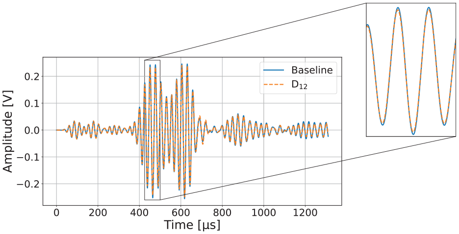
Comparison of a baseline measurement with a signal recorded when damage was applied (D₁₂). Even in the enlarged section, only a slight attenuation can be noticed.

Figure 7 shows the difference between a baseline signal and one with a hole in the surface between the actuator and sensor. After the electromagnetic crosstalk, which is again identical in both cases, an attenuation can be recognized in the event of damage.

A very small phase shift to the right only appears in some time ranges. Through analysis of the previously presented signals (Figures 4 –7) and comparisons with various additional signals, we can conclude that variations in temperature and load have a greater impact on guided waves than damage does.

Figure 6.

Varying pressure. In the magnified part of the plot, a phase shift to the left can be detected for higher pressures.

Figure 7.

Comparison of a baseline measurement with a signal recorded after the first hole was drilled $({RD}_{1}^{V})$ . In the enlarged section, a slight attenuation and a small phase shift to the right at some points can be seen.

Methodology

In this section, the methods developed in this work are introduced. A brief overview of the metrics relevant to the following sections is provided at the beginning. Afterward, two different ways of converting the measured signals into representations that serve as input for the utilized classification algorithms are presented. These include the GAF, which generates an image-like matrix, as well as the features calculated by a time series feature extraction method called MiniRocket.²⁸

The two classification models belonging to the field of supervised learning – CNN and RRC – are shown next. While the GAFs are interpreted by a CNN, a comparatively simpler RRC uses MiniRocket features.

This is followed by a description of the anomaly detection algorithm called LOF, which is an unsupervised learning method that does not require signals from a damaged structure for training.

Lastly, it is explained how ensemble voting combines the predictions of individual actuator-sensor pairs. This approach makes it possible to obtain a collective prediction for the entire system and significantly improves the accuracy compared to the individual predictions. The procedure for an optimal choice of the decision threshold, which is used to distinguish between damaged and undamaged, is explained in the last part of the section.

Metrics

For classification tasks in ML, there are a few particularly important metrics that appear at various stages. These are relevant both for training when optimizing the hyperparameters and selecting the decision threshold as well as for evaluating the performance of the models when used on test data.

A common method for measuring the performance of a classifier and analyzing the kinds of errors it makes is the so-called confusion matrix. It is shown for two classes in Figure 8: undamaged is labeled as 0, damaged as 1. For a perfect classification model, the predicted labels always match the actual labels. This means that there are only true negatives (TNs) and true positives (TPs). If, on the other hand, the real label for a signal does not correspond to the one output by the classification model, the error can be characterized as a false negative (FN) or false positive (FP).

Figure 8.

Confusion matrix for two categories.

Accuracy refers to the proportion of correct predictions out of all predictions. The precision value describes the ratio of correct positive predictions to all positive predictions. Also known as sensitivity or true-positive rate (TPR), recall is calculated as the percentage of positive instances that are correctly classified. The previous two metrics can be combined using the harmonic mean into a single metric called F₁ score, which allows for easier comparison of multiple classifiers. Using the harmonic mean as opposed to the arithmetic mean, low scores are given much more weight. As a result, high scores can only be achieved if both precision and recall are good, especially if they are similar.

$accuracy = \frac{TP + TN}{TP + TN + FP + FN}$ (1)

$precision = \frac{TP}{TP + FP}$ (2)

$recall = \frac{TP}{TP + FN}$ (3)

$F_{1} = \frac{2 TP}{2 TP + FP + FN}$ (4)

The so-called receiver operating characteristic (ROC) shows the relationship between the TPR (equivalent to recall) and the false-positive rate (FPR). As with precision and recall, one of the two metrics generally gets worse when the other gets better. A simple way to assess the performance of a classifier is the area under the curve (AUC), which is 0.5 for a random classifier and 1.0 for a perfect one.

$TPR = \frac{TP}{TP + FN}, FPR = \frac{FP}{FP + TN}$ (5)

Data preprocessing

Depending on the choice of the classification model, the data must be prepared in different ways. The two approaches used for data pre-processing in this work are GAF and MiniRocket.

Gramian angular field

Previous research of this paper’s authors successfully investigated transforming UGW into mel-frequency cepstral coefficients matrices, a compressed form of a spectrogram retaining information about time and frequency, for detecting damage and estimating its size and location.^29–31 One of the aims of this work was to find further forms of image-like matrices for the utilization of a CNN. While previous approaches focused on a dataset of OGW without environmental influences, this study’s classification tasks take temperature fluctuations into account.

In initial tests on this dataset, GAF achieved more promising results than recurrence plots and Markov transition fields (MTF). An overview of the different approaches with imaging methods in TSC, in general, can be found in Ismail Fawaz et al.,³² a recent application of GAFs specifically in the field of SHM in Liao et al.³³

GAFs (and MTFs) were proposed in 2015 by Zhiguang Wang and Tim Oates as a new method for encoding time series as images.^34,35 These are described using polar coordinates as a Gramian matrix whose elements represent the trigonometric sum of different time intervals.

First, the time series $X = {x_{1}, x_{2}, \dots, x_{n}}$ is normalized to the interval [−1,1] or [0,1].

${\tilde{x}}_{- 1}^{i} = \frac{(x_{i} - \max (X) + (x_{i} - \min (X))}{\max (X) - \min (X)}$ (6)

${\tilde{x}}_{0}^{i} = \frac{x_{i} - \min (X)}{\max (X) - \min (X)}$ (7)

Next, the transformation into polar coordinates is done by encoding the value as the angular cosine and the time stamp as the radius.

${\begin{matrix} ϕ = \arccos ({\tilde{x}}_{i}), - 1 \leq {\tilde{x}}_{i} \leq 1, \tilde{x} \in \tilde{X} \\ r = \frac{t_{i}}{N}, t_{i} \in N \end{matrix}$ (8)

Here, t_i refers to the time stamp and N to a constant for the regularization of the span of the polar coordinate system. The encoding is followed by the conversion to the GAF, where a distinction is made between the Gramian angular summation field (GASF) and the Gramian angular difference field (GADF).

$GASF = [\begin{matrix} \cos (ϕ_{1} + ϕ_{1}) & \dots & \cos (ϕ_{1} + ϕ_{n}) \\ \cos (ϕ_{2} + ϕ_{1}) & \dots & \cos (ϕ_{2} + ϕ_{n}) \\ ⋮ & ⋱ & ⋮ \\ \cos (ϕ_{n} + ϕ_{1}) & \dots & \cos (ϕ_{n} + ϕ_{n}) \end{matrix}]$

$= {\tilde{X}}^{'} \cdot \tilde{X} - {\sqrt{I - {\tilde{X}}^{2}}}^{'} \cdot \sqrt{I - {\tilde{X}}^{2}}$ (9)

$GADF = [\begin{matrix} \sin (ϕ_{1} - ϕ_{1}) & \dots & \sin (ϕ_{1} - ϕ_{n}) \\ \sin (ϕ_{2} - ϕ_{1}) & \dots & \sin (ϕ_{2} - ϕ_{n}) \\ ⋮ & ⋱ & ⋮ \\ \sin (ϕ_{n} - ϕ_{1}) & \dots & \sin (ϕ_{n} - ϕ_{n}) \end{matrix}]$

$= {\sqrt{I - {\tilde{X}}^{2}}}^{'} \cdot \tilde{X} - {\tilde{X}}^{'} \cdot \sqrt{I - {\tilde{X}}^{2}}$ (10)

In the last step, I was used as the unit row vector $[1, 1, \dots, 1]$ . With the definition of the inner product $< x, y > = x \cdot y - \sqrt{1 - x^{2}} \cdot \sqrt{1 - y^{2}}$ and $< x, y > = \sqrt{1 - x^{2}} \cdot y - x \cdot \sqrt{1 - y^{2}}$ , the GAF types can also be written as quasi (the defined functions do not satisfy the linearity criterion) Gramian matrices.

An implementation of the algorithm for generating the GADF and GASF matrices is available in the Python package pyts.³⁶ The parameters used in this work can be found in the section “Results.”Figure 9 shows an example of how a signal from the OGW dataset is transformed into GAF matrices of size $128 \times 128$ .

Figure 9.

After normalization of a signal from OGW, the transformation into polar coordinates follows. The GASF and GADF matrices are reduced to the size $128 \times 128$ using PAA.

MiniRocket

MiniRocket was recently introduced by Dempster et al.²⁸ It is an almost deterministic variant of Rocket and up to 75 times faster for large datasets than its already comparatively quick predecessor. Thanks to these improvements, there is currently no TSC algorithm that has such low computational cost with the same level of accuracy.

In a nutshell, MiniRocket works as follows: By default, 10,000 kernel-dilation-bias combinations are used to perform convolutions with a time signal. This is followed by the calculation of the proportion of positive values (PPV), a type of pooling for dimensionality reduction. These values between 0 and 1 form the features that are then used to train a linear classifier. For datasets with fewer than 10,000 time series, the authors recommend an RRC, for larger datasets a logistic regressor. However, in the section “Results,” it is shown that these features can also be successfully used for other models, in particular for an anomaly detection algorithm, which is introduced in the section “Local outlier factor.”

The application of a kernel $ω$ with dilation d and bias b to a time series X is given by:

$Z_{i} = X_{i} * ω = (\sum_{j = 0}^{l_{kernel} - 1} X_{i + (j \cdot d)} \cdot ω_{j}) + b$ (11)

Specifically, in the context of guided waves, X is the ultrasonic signal and $X_{i}$ is the single sample.

Only the PPV is then of relevance for MiniRocket.

$PPV (Z) = \frac{1}{n} \sum_{i = 0}^{n - 1} [Z_{i} > 0]$ (12)

An implementation of the algorithm is available in the Python package sktime.³⁷

Classifiers

The following section presents three approaches for using features derived from measured signals in classification. The first is the RRC, which takes the MiniRocket features as input. Next is the CNN, which is trained with GAF matrices. These two methods are supervised learning techniques, utilizing labeled data for training. The third approach is the LOF, an unsupervised learning technique that does not require labeled data. Again, MiniRocket features are used as input.

Ridge regression classifier

Linear models are characterized by the fact that they make predictions using a weighted sum of the input features plus a constant called the bias term or intercept term. The notation is based on Géron³⁸

$\hat{y} = θ_{0} + θ_{1} x_{1} + θ_{2} x_{2} + \dots + θ_{n} x_{n} = θ^{T} x$ (13)

Here, $\hat{y}$ is the predicted value, n the number of features, and $x_{i}$ the $i th$ feature and $θ_{j}$ the $j th$ model parameter.

$MSE (θ) = \frac{1}{m} \sum_{i = 1}^{m} {(θ^{T} x^{(i)} - y^{(i)})}^{2}$ (14)

During the training of the model, its parameters are set to predict training set values as accurately as possible, typically measured using the root mean square error (MSE). In practice, however, the MSE is used instead, which leads to the same minimum, as the root function is monotonically increasing.

Regularization methods like ridge regression, also known as Tikhonov regularization, can be used to prevent overfitting by adding a regularization term to the cost function $J (θ)$ . In this way, the model is designed to simultaneously minimize the deviation from the training data and keep the weights as small as possible.

$J (θ) = MSE (θ) + α \frac{1}{2} \sum_{i = 1}^{n} θ_{i}^{2}$ (15)

The strength of the regularization depends on the hyperparameter $α$ . For $α = 0$ , the cost function equals that of linear regression. For large values of $α$ , all weights become very small, which produces a flat line through the data’s mean.

While regression is normally applied to predict continuous values, it can also be used for classification with scikit-learn’s RidgeClassifier, which converts target labels to {−1, 1} and minimizes the cost function as described above. The sign of the model’s output determines the class of the analyzed instance. RidgeClassifierCV, which is used in this work, additionally implements leave-one-out cross-validation to optimize $α$ within a given range.

Convolutional neural network

The CNN used here was the so-called EfficientNetV2,³⁹ which was chosen for its impressive balance of size and performance. As a small model, it offers the advantages of minimizing hardware requirements, reducing training time and lowering the risk of overfitting due to limited training data. While a small CNN (about 640,000 parameters) inspired by Géron³⁸ was successfully utilized in previous work,^29–31 initial tests proved this simple architecture to be insufficient for the more complex task involving environmental influences. Instead, the smallest variant (about 6 million parameters) of EfficientNetV2 was selected for this task. Specifically, keras_cv.models.EfficientNetV2B0Backbone()⁴⁰ was implemented, with a GlobalMaxPooling2D and a Dropout layer added as measures against overfitting and a Dense layer with softmax activation for predicting the two class probabilities.

The training of the network, initialized with random weights, was run on a T4 GPU on the cloud-based service Google Colab. Within 750 epochs, the loss function categorical cross-entropy was minimized with the Adam optimizer and the learning rate scheduler cosine decay. Details on hyperparameters and pre-processing of input data can be found in the section “Results.”

Local outlier factor

In a realistic SHM scenario, the damage can vary in size, severity, and number, but there is only one undamaged state (apart from environmental influences). In this situation, it is necessary to determine whether a new input belongs to the same distribution of known observations (inlier) or comes from a different one (outlier). This problem can be further subdivided into outlier detection and novelty detection.

In outlier detection, the training data are contaminated with a few outliers located in regions of low density that are to be found. Novelty detection, on the other hand, assumes that all data from the training set belong to the same class. If a new observation is labeled as an outlier, it is referred to as a novelty. In the context of damage detection, novelty detection is particularly interesting, as only undamaged signals are needed for training. This provides an important reduction in hardware requirements and experimental effort. However, outlier signals are still required to evaluate model performance.

For this work, the scikit-learn implementation of LOF²⁵ was selected for anomaly detection. LOF measures the extent to which the object under consideration can be described as an outlier. For objects deep in a cluster, the LOF value is approximately 1, as the densities of an object are comparable to those of its neighbors. Values significantly greater than 1, which indicate an outlier, are caused by the low densities of the object under consideration and the high densities of its neighbors. Very high values are therefore achieved when a single object is located far away from a cluster of high density.

An example with synthetic data for illustration of the method is shown in Figure 10. Three isotropic Gaussian clusters were created for part (a) of the figure using scikit-learn’s make_blobs function. The clusters with different standard deviations each contain 200 blue points. In addition to these, 20 red random points were included. Part (b) of the figure shows the categorization into inliers and outliers by the LOF algorithm. The size of the circles is proportional to the LOF score, which is displayed for outliers. As expected, the LOF scores are higher the more isolated the points are. A few of the random points that are very close to the clusters are incorrectly described as inliers, but the algorithm cannot be blamed for any obvious errors. The same applies to mistakes in which actual inliers are declared as outliers.

Figure 10.

Exemplary use of LOF on a synthetic dataset: (a) synthetic dataset. In addition to three clusters, 20 random points were inserted and (b) points marked with blue circles were identified as inliers by the LOF algorithm, red circles show outliers.

Collective predictions

In the previous sections, all the methods necessary for classification were presented. The next step is combining predictions from individual transducer pairs to significantly improve accuracy and provide a single prediction for the overall state of the test object, rather than just for a part of it.

Ensemble voting

The first part of the approach is simple to implement and is summarized in Figure 11. After choosing one of the three methods (CNN, RRC, and LOF), a model is trained for each of the 36 transducer pairs. Each model now predicts each new signal, outputting either 0 (undamaged) or 1 (damaged) for CNN and RRC, or −1 (outlier or damaged) or 1 (inlier, undamaged) for LOF. Next, the mean values of all predictions relating to the same signal are calculated. For example, if 27 of the 36 models predict damage, the average score would be $\frac{9 \cdot 0 + 27 \cdot 1}{36} = 0.75$ for CNN and RRC, or $\frac{9 \cdot 1 + 27 \cdot (- 1)}{36} = - 0.5$ for LOF. The decision threshold is typically set in the middle of the two possibilities. Accordingly, all averaged predictions above 0.5 (for CNN or RRC) or below 0 (for LOF) indicate damage. However, adjusting the threshold based on the dataset, as shown in the section “Results,” may improve the accuracy of the results.

Figure 11.

Flowchart illustrating ensemble voting.

Decision threshold

To determine a customized decision threshold, a sufficiently large dataset is necessary, as cross-validation requires signals of different labels and positions. However, cross-validation was not performed for the LOF algorithm, as this would have been contrary to the basic idea of using only baselines for training. Nonetheless, the same methodology could theoretically also be applied to LOF.

The process consists of several steps, summarized in Figure 12. First, a part of the dataset (the test set) is set aside to evaluate the method later. It is crucial for a realistic assessment of the model’s performance that the test data are not used for training or for optimizing any parameters. Here, the data for one of the four damage locations and a subset of the baselines were withheld.

Figure 12.

Flowchart for determining the ideal decision threshold for a given dataset.

Cross-validation follows as the second step. For this purpose, the main dataset (training–validation set) is divided into several segments. Two of the remaining three positions are used for training (training set), and the third position is for validation (validation set). This is done for all possible splits into training and validation sets, which in this case were three different ones.

Afterward, the training set is used to adjust the model weights and the validation set is used for the evaluation. Several metrics are calculated for the entire range of possible threshold values. The aim is to select the threshold value at which the F₁ score is maximized (more precisely, the midpoint of the range where the F₁ score is at its maximum). The average of the threshold values across the splits is then saved.

All of the previous steps were designed to find a suitable threshold value that hopefully works well for unknown data and especially signals of new damage locations. To examine this, the performance of a model trained on the entire training-validation set is now assessed on the test set that was retained for this purpose. This is accomplished by applying the threshold found with cross-validation and assigning one of the two possible labels to the averaged predictions for each signal of the test set.

Results

Results for temperature or load varying datasets are reported here. For the former case, the three approaches are tested and compared. In the latter case, the third approach is validated on a realistic damage scenario.

Temperature-varying dataset

(1) GAF and CNN

The first step was to optimize the most important settings for GAF and CNN through a hyperparameter search, which was carried out using only one transducer pair due to time constraints. For the paths (4–10) located in the middle of the CFRP plate, the validation accuracy was to be maximized. In doing so, it was important to include signals from other damaged locations in the validation set as otherwise achieving 100% accuracy would have been far too easy. In fact, even without optimized parameters, perfect metrics were obtained when the training and validation set differed only in temperature or measurement repetition number, but not in position. This suggests that the real challenge lies in detecting damage at previously unknown locations—a factor not always considered in the literature, though important for a performance assessment under more realistic conditions.

The hyperparameters search was performed with the optimization framework optuna.⁴¹ With its efficient TPESampler (tree-structured Parzen estimator) and MedianPruner, which stops the training of unpromising trials before all epochs are completed, time is saved. Nevertheless, optimization is still very time-consuming. In this case, 30 combinations of parameters were tested, with 11 fully executed and 19 pruned, taking about 5.5 h. The resulting hyperparameters are detailed in Table 1.

Table 1.

Hyperparameter optimization results for GAF + CNN.

Parameter	Value	Search range
GAF size	128	32, 64, 128
GAF type	Difference	Summation, difference
Standardization	False	True, False
Learning rate	1.29e-4	1e-5–5e-3
Alpha	0.1	1e-6, 1e-5, …, 0.0
Dropout rate	0.47	0.4–0.6

GAF: Gramian angular field; CNN: convolutional neural network.

Figure 13 shows the accuracy, precision, recall, and F₁ score metrics for the test set signals of the six channels under consideration. With 81 baselines and 161 damage signals in the test set, a CNN that always predicts undamaged would therefore have an accuracy of $\frac{81}{81 + 161} \approx 33 %$ . This is the case here with (3–10) and (5–12). For models trained on paths (2–7) and (6–11), nearly perfect results were achieved. At first glance, the average accuracy of the considered channels may seem discouraging for damage detection. However, as will be shown later, it is sufficient with the developed methodology if only a small proportion of classifiers perform well.

Figure 13.

Evaluation of predictions by the CNN for individual transducer pairs.

With the exception of (3–10), where no damage was detected and the precision is undefined, precision values for all channels are 100% or very slightly below. Therefore, if a CNN predicts damage, the test object is actually damaged. This property is crucial for the success of the ensemble voting. The recall plot shows that while two channels recognized almost all damages, two others detected almost none. Finally, the F₁ score combines all the findings, highlighting that in this case two of the six channels are basically of no use for damage detection.

The results shown so far were for individual CNNs. Now, the combination of their predictions is analyzed. After all, the aim is to generate an overall prediction of all trained classifiers.

Before the execution of ensemble voting, the optimal decision threshold must first be found. For this purpose, cross-validation was performed with various splits. Their individual metrics are not listed here, as only the optimized threshold is of interest.

Figure 14 illustrates the determination of the best threshold using one of the three cross-validation splits. In this example, training included positions D₀₄ and D₂₄ in addition to baselines, while validation was carried out with D₁₂ and other baselines. The x-axis shows the decision threshold, ranging from 0 to 1. On the y-axis, the four previously considered metrics are displayed. The decision threshold can be understood as the proportion of classifiers that must be reached for the ensemble to predict damaged. The step-like shape of the graphs is a result of the number of classifiers (six) and possible predictions (two) being finite. Since the mean values of the predictions in this case can only include values from the set ${\frac{0}{6}, \frac{1}{6}, \dots, \frac{6}{6}}$ , there are six horizontal segments in the plot, with the last three at the same height.

Figure 14.

For the validation set, a decision threshold value of 0.083 maximizes the F₁ score for the CNN approach.

The metrics reach their minimum at a threshold above 0.5 or are undefined in the case of precision. The vertical dotted line indicates the center of the section in which the F₁ score is at its maximum. This value of 0.083 was also found for the other two splits. However, the lowest threshold is not always best, as shown later with MiniRocket, where a larger number of classifiers was used.

Figure 15 then shows the metrics for the test set. Compared to the previous plot, all metrics are now significantly better for the majority of possible threshold values. This is probably due to the fact that the entire training-validation set was used for training, giving the CNNs more examples to learn to distinguish between damaged and undamaged. The dotted line is the optimized threshold found in the cross-validation. In this case, all values below 0.33 would have led to perfect results, including the cross-validated threshold applied here. However, which thresholds are optimal can only be known in hindsight. If the best threshold were selected based on Figure 15, no realistic performance measurement would be possible. When the classification system is actually deployed, for example, two out of six classifiers could result in damaged. Whether the overall prediction should be undamaged or damaged depends on the threshold, which must be set before testing or real-world use.

(2) MiniRocket + RRC

Figure 15.

Various metrics versus threshold for the test set using the CNN approach.

For the second method, MiniRocket transformed the signals and an RRC classified them. The procedure was similar to the previous one but with 36 transducer pairs and a broader range of scenarios. First, however, the hyperparameters to be set are briefly discussed.

MiniRocket’s hyperparameter search is straightforward, as only the number of kernels (num_kernels) significantly impacts the results. The best way to optimize this parameter was to look at the threshold plots for different values. It quickly became clear that far fewer than the 10,000 kernels specified as the standard in the original paper were required. An amount of 500 proved sufficient and even outperformed models with more kernels, as can be seen in Figure 16.

Figure 16.

Optimization of the num_kernels hyperparameter with the RRC approach. (a) 250 kernels, (b) 500 kernels, and (c) 750 kernels.

The criterion for a suitable value of the num_kernels hyperparameter was the width of the region in which the F₁ score equals 1 on the curves shown in Figure 16. The idea is that when the averaged predictions for damaged and undamaged are far apart, the ensemble can distinguish well between the classes. For 250 kernels, the metrics get worse (i.e., the ensemble of classifiers makes more errors) for small thresholds, but decrease more slowly for larger thresholds. For 750 kernels, the metrics are perfect for small thresholds but drop quickly for larger thresholds. Therefore, a value of 500 kernels offers a good compromise with a wide range of optimal metrics.

Aside from $random_state = 42$ for reproducibility, sktime’s default MiniRocket implementation settings were used. For scikit-learn’s RRC, alpha was set to numpy.logspace (−3, 3, 10),⁴² as it is done in sktime’s RocketClassifier.

In direct comparison to the CNN, the scores for the channels used in both methods are slightly higher on average for the RRC. More important, however, is the performance of the ensemble, which is shown in Figure 17 for D₁₆. The threshold value optimized with cross-validation and marked with a dotted line lies in a range that enables perfect metrics. The same holds true for D₀₄ and D₂₄. For D₁₂, the threshold is slightly too large, so that “only” 99.6% accuracy is achieved.

(3) MiniRocket + LOF

Figure 17.

Various metrics versus threshold for damage location D₁₆ in the test set using the RRC approach.

This anomaly detection approach aimed to use only baselines for the training data. The first three-quarters of all baselines were included in the training set, while the last quarter and the data for the CFRP plate damaged at one position formed the test set. This procedure was followed for all four damaged positions, resulting in four test sets. As done by Dempster et al.²⁷ and Tu et al.,⁴³ where unsupervised learning methods were also used for SHM, AUC was selected as the key metric for the evaluation of the model.

First, the hyperparameters were optimized utilizing the D₀₄ signals for validation, to maximize the mean AUC value of all channels. Unfortunately, optimization with baselines alone is not possible, as the evaluation of predictions for actual anomalies is essential for performance assessment. Table 2 shows the values of the hyperparameters found, including the number of kernels for MiniRocket as well as the number of neighbors and contamination for LOF. The variation of n_neighbors led to the largest fluctuations in the target metric, contamination had comparatively little influence.

Table 2.

Hyperparameter optimization results for MiniRocket + LOF using the OGW dataset.

Parameter	Value	Search range
num_kernels	5000	100–10,000
n_neighbors	6	1–42
Contamination	0.004	0.001–0.2

OGW: open-guided waves; LOF: local outlier factor.

Figure 18 illustrates the AUC values for D₁₂, which had the worst performance of the four damaged locations. It is possible that the aluminum disk at this position was not as strongly attached to the test object as the others, making it slightly more difficult to detect. Still, a mean AUC of 91% across all transducer pairs was achieved. Even if no absolute rule can be determined, it can still be seen that greater distances result in weaker classification results.

Figure 18.

AUC for detecting damage at position D₁₂ with the 36 paths of the OGW dataset considered with LOF.

The threshold plots in Figure 19 look slightly different than before due to LOF returning either −1 or 1 as a prediction. While 1 means damaged for CNNs and RRCs, 1 here indicates inlier, that is, undamaged. Despite this difference, the analysis proceeds similarly with one notable change: the averages were weighted with $e^{a}$ , where a is the anomaly score, which increases the more confident the model is that it recognizes damage. This means that not all transducer pairs are equally important in ensemble voting. As damage is most likely detected for paths near the damage, the influence of these predictions could be too small with a simple unweighted mean value, especially when monitoring large surfaces. Although for all damage locations optimal metrics are achieved for small sections even without this additional step, weighting broadens the range of threshold values with optimal performance, making the distinction between inliers and outliers more robust.

Figure 19.

Various metrics versus threshold for damage location D₁₂ in the test set using LOF with and without weighted averages. (a) With weighting and (b) Without weighting.

Lastly, Table 3 presents the compiled results for the three methods. For GAF + CNN and MiniRocket + RRC (MR + RRC), both the average accuracies across all transducer pairs and the ensemble accuracies are reported. For MiniRocket + LOF (MR + LOF), the AUC values are displayed to represent the method’s performance. Regardless of the damage location selected, the ensembles of all three methods reliably distinguished between the two classes for nearly all signals and temperatures. Given that UGW signals contain multi-modal dispersive waveforms with reflections—such as those from structural boundaries—along with signal changes resulting from temperature and load variations, this unpredictable behavior limits the applicability of ML methods when considering new transducer pairs that were not included in the training phase (Table 3).

Table 3.

Results of all methods.

Method	Loc.	Metric	Mean	Ensemble
GAF + CNN	$D_{16}$	acc.	0.68	1
MR + RRC	$D_{04}$	acc.	0.54	1
	$D_{12}$	acc.	0.46	0.996
	$D_{16}$	acc.	0.61	1
	$D_{24}$	acc.	0.61	1
MR + LOF	$D_{04}$	AUC	0.95	1
	$D_{12}$	AUC	0.91	1
	$D_{16}$	AUC	0.97	1
	$D_{24}$	AUC	0.96	1

GAF: Gramian angular field; CNN: convolutional neural network; MR: MiniRocket; RRC: ridge regression classifier; LOF: local outlier factor; AUC: area under the curve.

Load-varying dataset

Addressing real-world situations, we found that the application of supervised ML approaches was not feasible, as the vessel could only be destroyed once. Therefore, this study explores the applicability of unsupervised methods in this practical scenario. First, the hyperparameters are optimized to maximize the average AUC value across 15 transducer pairs considered for the analysis (paths having either transducer #6 or transducer #16 enabled). During the hyperparameter optimization, the first half of the baselines (i.e., the three repetitions of the first pressure ramp, corresponding to a total of 42 signals per transducer pair) was used for training, the second half of the baselines and the data for $D_{1}^{V}$ (a total of 126 signals per transducer pair) for validation. Table 4 shows the optimized number of kernels for the MiniRocket transformations, number of neighbors, and contamination for the LOF classifier.

Table 4.

Hyperparameter optimization results.

Parameter	Value	Search range
num_kernels	2500	100–10,000
n_neighbors	3	1–42
Contamination	0.03	0.001–0.2

The results after the application of the ensemble voting process are summarized as ROC curves in Figure 20. For $D_{1}^{V}, D_{4}^{V}$ and ${RD}_{4}^{V}$ , perfect AUC values were achieved. The only deviation from the optimal curve is found for ${RD}_{1}^{V}$ . With an AUC value of 0.74, which presents a considerable difference between detection of single artificial and real damage. Apparently, the glued steel blocks were easier to detect than an actual hole. The performance of an SHM system could therefore be overestimated if it was only tested with (too large) artificial damages beforehand. Therefore, the results highlight how important but also difficult it is to simulate realistic conditions as accurately as possible. Since LOF is an unsupervised learning method, no signals for damaged objects are needed in training, which minimizes the experimental effort. However, a small data set for damages would be beneficial for tuning hyperparameters and the decision threshold to the specific use case as well as for measuring reliability.

Figure 20.

ROC curves and AUC values when applying the method to ideal and real damage.

Discussion

Comparison between supervised learning methods

The first two methods are fundamentally similar in their application, which simplifies comparison. Both require labeled data from both undamaged and damaged test objects for training and classify transformed signals into one of two categories. The primary objective of this study is to develop a robust ML model (supervised, unsupervised) for detecting damage to structures under varying environmental and operational conditions, specifically temperature and load. Beyond the slightly higher classification accuracy for individual transducer pairs, several other advantages favor MiniRocket + RRC. The most obvious is the significantly shorter training time for MiniRocket—only a few seconds per transducer pair compared to around 15 min for the CNN. This makes it possible to consider significantly more channels, which generally leads to more reliable classifications, as it allows for better coverage of the monitored object’s surface. Moreover, malfunctions of single transducers are less problematic since neighboring transducers still observe similar segments. Another advantage is the lower hardware requirements for the RRC compared to the CNN, which needs a GPU for efficient training, whereas a CPU is sufficient for the RRC. In addition, the reproducibility of the results of the MiniRocket + RRC method helps in comparing different approaches. The simpler hyperparameter optimization, in which only the number of convolutional kernels needs to be varied, is also worth mentioning. Finally, MiniRocket and in particular sktime’s RocketClassifier are more user-friendly, requiring less prior knowledge and being applied faster thanks to existing implementations.

In its current form, the verdict is therefore clearly in favor of MiniRocket + RRC. However, the number of possible variations of the CNN approach is so large that it should not yet be ultimately dismissed.

Supervised versus unsupervised learning approaches

After ensemble voting, the supervised learning approach almost always achieved perfect results, thanks to excellent precision values from individual transducer pairs and the ability to optimize decision thresholds using data from various damage locations. Another advantage of this approach is the large number of classifiers for which there are already implementations that can potentially be tested in the future.

However, signals from structural damage at various positions are needed for a robust classifier with optimized hyperparameters and thresholds. Besides reversible damages like the aluminum disk attached to the CFRP plate for OGW, simulated damages could be an alternative to obtain a sufficiently large training set.

The unsupervised learning algorithm LOF is as easy to implement and fast as the RRC method. It also offers the major advantage of not requiring damaged object signals for training, greatly reducing the experimental workload. By distinguishing between inlier and outlier, a high performance of the individual classifiers and a strong correlation between AUC and proximity to damage is achieved. This makes a future use for localization in addition to classification feasible, with anomaly scores increasing the closer the damage is to the transducer pair.

However, there are also downsides such as how to interpret the results when no threshold is determined beforehand. One option is to check anomaly scores of new or retained baselines, classifying anything below the lowest value for the undamaged object as outliers. Alternatively, a threshold simply set at 0.0 would have achieved very good results for this dataset. While real damages would probably be more appropriate for determining a decision threshold, this would to some extent contradict the original goal of using only baselines for training and still require actual damages to assess realistic performance.

Considering the strong performance of the individual classifiers, the wide ranges for threshold values, with which (almost) perfect metrics are achieved, as well as the potential for damage localization, especially considering the anomaly score, there are many arguments for continuing research with the LOF approach. In future work, we will consider experimental signals corresponding to specific temperature ranges, designated as test data to facilitate an unbiased evaluation of the model’s performance. The ML models will be trained on data collected from conditions that do not include these observations from the specified test temperature and load ranges. This methodology is intended to assess the models’ generalizability and performance under previously untested environmental and operational conditions. Furthermore, we plan to broaden the range of environmental conditions by conducting new measurements over a pressure vessel that will test the performance of the studied ML models across a spectrum of simultaneous temperature and load variations which will further validate the models’ generalizability and robustness.

Conclusion

The paper demonstrated the performance of supervised and unsupervised ML methods in the context of damage detection in the presence of temperature or load variations, resembling the operational conditions of the specimens. The main results of this work can be summarized as follows:

The supervised learning algorithms RRC and CNN were implemented and tested alongside the unsupervised learning algorithm LOF to successfully identify damage in a CFRP plate under varying temperature or load conditions.

Both time series transformation methods, GAF and MiniRocket, provided suitable and valuable features for the ML models, accurately reflecting the state of the structure. MiniRocket, which was applied for the first time in the context of SHM with UGW, combined with RRC or LOF, proved to be the most time-efficient approach used in this study.

Ensemble Voting significantly improved the reliability of damage detection by combining predictions from multiple transducer pairs. Even with a limited number of strong individual classifiers, 100% accuracy was achieved in most cases.

The combined approach of MiniRocket, supervised/unsupervised ML algorithms, and ensemble voting proved to be an effective, hardware- and time-efficient strategy for detecting damage in the composite structure. This approach successfully overcame the challenges introduced by temperature or load variations, even in locations not included in the training of the ML models.

Footnotes

The authors gratefully acknowledge financial support by the German Federal Ministry for Education and Research (BMBF) under grant number 03VP10461 within the project “Künstliche Intelligenz für das Ultraschall-Monitoring von Wasserstoff-Druckbehältern” (KIMono). In addition,the authors would like to express our gratitude for the valuable technical discussions with partners from the KIMono project,specifically those from Fraunhofer IKTS and the University of Saarland,whose insights contributed to the development of this study.

Declaration of conflicting interests

The author(s) declared no potential conflicts of interest with respect to the research,authorship,and/or publication of this article.

Funding

The author(s) disclosed receipt of the following financial support for the research,authorship,and/or publication of this article: This work was supported by the German Federal Ministry for Education and Research (BMBF) [grant number 03VP10461].

Ethical considerations

This article does not contain any studies with human or animal participants.

Consent to participate

There are no human participants in this article and informed consent is not required.

ORCID iDs

Oliver Schackmann

Octavio A. Márquez Reyes

Jochen Moll

References

De Simone

Lorusso

Santaniello

Predictive maintenance and structural health monitoring via IoT system. In: 2022 IEEE workshop on complexity in engineering (COMPENG), Florence, Italy, 2022, pp. 1–4.

Yang

Tian

, et al. A review on guided-ultrasonic-wave-based structural health monitoring: From fundamental theory to machine learning techniques. Ultrasonics 2023; 133: 107014.

Cusati

Corcione

Memmolo

. Potential benefit of structural health monitoring system on civil jet aircraft. Sensors 2022; 22(19): 7316.

Ballarin

Macchi

Roda

, et al. Economic impact assessment of structural health monitoring systems on helicopter blade beginning of life. Struct Control Health Monit 2024; 2024(1): 2865576.

Gorgin

Luo

. Environmental and operational conditions effects on lamb wave based structural health monitoring systems: a review. Ultrasonics 2020; 105: 106114.

Croxford

Moll

Wilcox

, et al. Efficient temperature compensation strategies for guided wave structural health monitoring. Ultrasonics 2010; 50(4–5): 517–528.

Moll

Kexel

Pötzsch

, et al. Temperature affected guided wave propagation in a composite plate complementing the Open Guided Waves Platform. Sci Data 2019; 6(1): 191.

Dobson

Cawley

. Independent component analysis for improved defect detection in guided wave monitoring. Proc IEEE 2015; 104: 1620–1631.

Ren

Giannakeas

Sharif Khodaei

, et al. Theoretical and experimental investigation of guided wave temperature compensation for composite structures with different thicknesses. Mech Syst Signal Process 2023; 200: 110594.

10.

Maack

Brandt

Koerdt

, et al. Continuous baseline update using recurrence quantification analysis for damage detection with guided ultrasonic waves. Eur Phys J Special Topics 2023; 232(1): 179–185.

11.

Rheinfurth

Schmidt

Döring

, et al. Air-coupled guided waves combined with thermography for monitoring fatigue in biaxially loaded composite tubes. Compos Sci Technol 2011; 71(5): 600–608.

12.

Luca

Perfetto

Caputo

, et al. Numerical simulation of guided waves propagation in loaded composite structures. In: AIP Conference proceedings, 2020, vol. 2309. AIP Publishing.

13.

Chen

Wilcox

. The effect of load on guided wave propagation. Ultrasonics 2007; 47(1): 111–122.

14.

Gandhi

Michaels

Lee

. Acoustoelastic lamb wave propagation in biaxially stressed plates. J Acoust Soc Am 2012; 132(3): 1284–1293.

15.

Moix-Bonet

Schmidt

Eckstein

, et al. A composite fuselage under mechanical load: a case study for guided wave-based SHM. In: Proceedings of the 10th European workshop on structural health monitoring (EWSHM 2024), e-Journal of Nondestructive Testing, 2024, vol. 29.

16.

Brettschneider

Kraemer

. Analytical and experimental analysis of guided waves in an aluminum plate under bending load. Ultrasonics 2024; 141: 107324.

17.

Abbassi

Römgens

Tritschel

, et al. Evaluation of machine learning techniques for structural health monitoring using ultrasonic guided waves under varying temperature conditions. Struct Health Monit 2023; 22(2): 1308–1325.

18.

Le Bourdais

Mesnil

d’Almeida

. Machine-learning based temperature compensation for guided wave imaging in structural health monitoring. In: 11th International symposium on NDT in aerospace, Paris-Saclay, France (AeroNDT 2019), Nov 2019, vol. 25.

19.

Bao

Yang

, et al. Guided-wave-based real-time damage detection in composite structures: a Gramian angular field image coding lightweight network approach. IEEE Trans Instrumen Meas 2025; 74: 1–12.

20.

Rautela

Senthilnath

Moll

, et al. Combined two-level damage identification strategy using ultrasonic guided waves and physical knowledge assisted machine learning. Ultrasonics 2021; 115: 106451.

21.

Moll

Fritzen

. Guided waves for autonomous online identification of structural defects under ambient temperature variations. J Sound Vibr 2012; 331(20): 4587–4597.

22.

Bansal

Garg

. Environmental sound classification: a descriptive review of the literature. Intell Syst Appl 2022; 16: 200115.

23.

de Rezende

SWF

de Moura

JdRV

Neto

RMF

, et al. Convolutional neural network and impedance-based SHM applied to damage detection. Eng Res Express 2020; 2(3): 035031.

24.

Sen

Nagarajaiah

. Data-driven approach to structural health monitoring using statistical learning algorithms. In: Mechatronics for cultural heritage and civil engineering, 2018, pp. 295–305.

25.

Breunig

Kriegel

, et al. LOF: identifying density-based local outliers. In: Proceedings of the 2000 ACM SIGMOD international conference on management of data, Dallas, Texas, 15–18 May 2000, pp. 93–104.

26.

Barandas

Folgado

Fernandes

, et al. TSFEL: time series feature extraction library. SoftwareX 2020; 11: 100456.

27.

Wang

Zhang

Shen

, et al. Defect detection in guided wave signals using nonlinear autoregressive exogenous method. Struct Health Monit 2022; 21(3): 1012–1030.

28.

Dempster

Schmidt

Webb

. Minirocket: a very fast (almost) deterministic transform for time series classification. In: Proceedings of the 27th ACM SIGKDD conference on knowledge discovery & data mining, Singapore, 14–18 August 2021, pp. 248–257.

29.

Memmolo

Moll

Schackmann

, et al. Promoting novel strategies for the reliability assessment of guided wave based SHM systems. In: Structural health monitoring 2023 designing SHM for sustainability, maintainability, and reliability, 2023.

30.

Schackmann

Memmolo

Moll

. A unified CNN approach for guided wave-based damage detection, damage size estimation and reliability assessment demonstrated on a complex composite structure. Smart Mater Struct 2024; 33(10): 105034.

31.

Volovikova

Freitag

Schackmann

, et al. Artificial intelligence-based approach for damage localization in ultrasonic guided wave-based structural health monitoring. Preprints NDTnet 2024 2(2): 31–44.

32.

Ismail Fawaz

Forestier

Weber

, et al. Deep learning for time series classification: a review. Data Mining Knowledge Discovery 2019; 33(4): 917–963.

33.

Liao

Qing

Wang

, et al. Damage localization for composite structure using guided wave signals with Gramian angular field image coding and convolutional neural networks. Compos Struct 2023; 312: 116871.

34.

Wang

Oates

. Encoding time series as images for visual inspection and classification using tiled convolutional neural networks. In: Workshops at the twenty-ninth AAAI conference on artificial intelligence.

35.

Wang

Oates

. Imaging time-series to improve classification and imputation. arXiv preprint arXiv: 150600327, 2015.

36.

Faouzi

Janati

. Pyts: a python package for time series classification. J Mach Learn Res 2020; 21(46): 1–6.

37.

Löning

Bagnall

Ganesh

, et al. Sktime: a unified interface for machine learning with time series. arXiv preprint arXiv:190907872, 2019.

38.

Géron

. Hands-on machine learning with Scikit-Learn, Keras, and TensorFlow. Sebastopol, CA: O’Reilly Media, Inc. 2019.

39.

Tan

. Efficientnetv2: smaller models and faster training. In: 38th International conference on machine learning, virtual, 2021, pp. 10096–10106. PMLR.

40.

Chollet

Allaire

Brock

, et al. Keras. https://keras.io, 2015.

41.

Akiba

Sano

Yanase

, et al. Optuna: a next-generation hyperparameter optimization framework. In: Proceedings of the 25th ACM SIGKDD international conference on knowledge discovery and data mining, 2019.

42.

Harris

Millman

van der Walt

, et al. Array programming with NumPy. Nature 2020; 585(7825): 357–362.

43.

Pyle

Croxford

, et al. Potential and limitations of NARX for defect detection in guided wave signals. Struct Health Monit 2023; 22(3): 1863–1875.

Machine learning strategies with ensemble voting for ultrasonic damage detection in composite structures under varying temperature or load conditions

Abstract

Keywords

Introduction

Related works

Machine learning methods

Time series classification

Experimental data acquisition and generation of datasets

First experimental setup (OGW)

Second experimental setup (COPV)

Influence of temperature and load on UGW signals

Methodology

Metrics

Data preprocessing

Gramian angular field

MiniRocket

Classifiers

Ridge regression classifier

Convolutional neural network

Local outlier factor

Collective predictions

Ensemble voting

Decision threshold

Results

Temperature-varying dataset

Load-varying dataset

Discussion

Comparison between supervised learning methods

Supervised versus unsupervised learning approaches

Conclusion

Footnotes

Declaration of conflicting interests

Funding

Ethical considerations

Consent to participate

ORCID iDs

References