Sage Journals: Discover world-class research

Abstract

There is growing interest in imputing missing data in tabular datasets using deep learning. Existing deep learning–based imputation models have been commonly evaluated using root mean square error (RMSE) as the predictive accuracy metric. In this article, we investigate the limitations of assessing deep learning–based imputation models by conducting a comparative analysis between RMSE and alternative metrics in the statistical literature including qualitative, predictive accuracy, statistical distance, and descriptive statistics. We design a new aggregated metric, called reconstruction loss (RL), to evaluate deep learning–based imputation models. We also develop and evaluate a novel imputation evaluation methodology based on RL. To minimize model and dataset biases, we use a regression imputation model and two different deep learning imputation models: denoising autoencoders and generative adversarial nets. We also use two tabular datasets from different industry sectors: health care and financial. Our results show that the proposed methodology is effective in evaluating multiple properties of the deep learning–based imputation model’s reconstruction performance.

Keywords

Imputation missing data deep learning model checking evaluation metrics

Impact Statement

Missing data are a common challenge in health analytics due to the technical and privacy challenges in collecting medical records. There is growing interest in imputing missing data in health datasets using deep learning. Existing deep learning–based imputation models have been commonly evaluated using root mean square error (RMSE), a predictive accuracy metric. In this article, we investigate the challenges of evaluating deep learning–based imputation models by conducting a comparative analysis between RMSE and evaluation metrics used in the statistical literature, including qualitative, predictive accuracy, statistical distance, and descriptive statistics metrics. To address these challenges, we design a new aggregated metric to evaluate deep learning–based imputation models called reconstruction loss (RL). We also present and evaluate a novel imputation evaluation methodology based on RL that researchers, system designers, and developers can use to develop predictive medical systems.

Introduction

Missing data are a common challenge when analyzing tabular datasets such as electronic medical records.^1,2 One approach to handle missing data is imputation where the missing data are estimated using observed values in the dataset. There is growing interest in using deep learning to estimate the missing data. Deep learning imputation models include denoising autoencoders (DAEs³), and generative adversarial nets (GANs⁴). Deep learning models have three advantages over statistical imputation models such as logistic regression, decision trees, predictive mean matching (PMM), and sequential regression.⁵ First, deep learning imputation can be used without making assumptions about the underlying distribution of the data. Next, missing data across multiple features can be estimated using a single imputation model. Finally, deep learning models can capture the latent structure of complex high-dimensional data (e.g. the correlation between demographics, medical history, and clinical outcomes in health records).⁶

An important task in imputing missing data is evaluating the performance of the imputation models.⁷ Imprecise models can produce misleading instances that impact the distribution of the groups being analyzed. The resulting discrepancies can impact a deep learning model’s performance.⁸ The following motivating scenario demonstrates the importance of evaluating imputation models.

The authors of this article are currently developing a decision support system (DSS) using deep learning that assesses a patient’s risk from radiation exposure due to medical imaging (MI).⁹ Our dataset has approximately 2.3 million imaging records from 340,525 patients over 10 years in four hospitals in Hamilton, Ontario, Canada. Due to technical and privacy challenges, we could access a subset of 18,875 DICOM (Digital Imaging and Communications in Medicine) headers. As a result, we need to impute the patients’ exposure in the remaining imaging records in the dataset using other features (e.g. body part). A common approach to estimating exposure is using mean values from the literature.^10,11 However, a previous study¹² demonstrated that mean values from the literature under-estimate patients’ exposure. The resulting discrepancies had a cascading effect on the performance of the deep learning model.

A commonly used metric to evaluate the quality of a deep learning imputation model is the root mean square error (RMSE) which measures the difference between the imputed values and their corresponding actual values.^3,4,13 RMSE is a performance evaluation metric. However, the goal of imputation in the statistical literature¹⁴ is to ensure the imputed data meets the underlying properties of the dataset (e.g. data variability and distribution) rather than achieve the best prediction accuracy as in deep learning.⁷

Preliminary results of this research are published in Boursalie et al.¹⁵ where we presented a comparative analysis of performance metrics to assess deep learning–based imputation models using the evaluation methodology commonly used in the literature. Two major contributions exclusively reported in this article are (1) our proposed methodology for evaluating deep learning–based imputation models and (2) an experimental study of the efficiency of our proposed evaluation methodology compared to the existing methodology commonly used in the literature.

Materials and methods

In this section, we review existing imputation models, their evaluation methodology and metrics, and present our proposed evaluation methodology.

Imputation models

Consider a matrix $D$ containing data for $i$ instances described by $j$ features. The objective of inferential statistics is to estimate population parameters $Q$ such as mean $(μ)$ , variance $(σ)$ , and regression coefficients $(θ)$ by calculating statistics $\hat{Q} = (\hat{u}, \hat{σ}, \hat{θ})$ from $D$ . $D$ can also be used to train deep learning models. However, $D$ may contain observed $(D_{(1)})$ and missing $(D_{(0)})$ data. Together, $D = (D_{(1)}, D_{(0)})$ is the matrix with complete data. The response matrix $R = (r_{i j})$ shows the locations of observed $(r_{i j} = 1)$ and missing values $(r_{i j} = 0)$ . The missing data pattern of $R$ ¹⁶ can be described as missing completely at random (MCAR) when the probability of data being missing depends only on the overall probability of data being missing $(ψ)$ . Data are missing at random (MAR) when the probability of missing data depends on $ψ$ and $D_{(1)}$ . Finally, data are missing not at random (MNAR) when the probability of missing data depends on $ψ$ , $D_{(1)}$ , and $D_{(0)}$ .

We can estimate missing data by drawing synthetic observations from the posterior distribution of the missing data, given the observed data and the process that generated the missing data. Formally, the posterior distribution is denoted as $P (D_{(0)} | D_{(1)}, R)$ . Rubin¹ demonstrated that $R$ and the process that generated the missing data are ignorable when data are MCAR or MAR. In these cases, the distribution of $D$ is assumed to be the same in $D_{(1)}$ and $D_{(0)}$ .¹ As a result, we can model the posterior distribution using the observed data and then use this model to create imputations for the missing data $(P (D_{(0)} | D_{(1)}, R) = P (D_{(0)} | D_{(1)}))$ . Note that we need to include $R$ and the process that generated the missing data in the model of the posterior distribution $(P (D_{(0)} | D_{(1)}, R))$ when data are MNAR.

Imputation models that estimate the posterior distribution of $D$ can be classified as non-generative or generative. Non-generative models include PMM¹⁷ and Multiple Imputation with Denoising Autoencoders (MIDAS¹³). PMM constructs separate multiple Bayesian linear regression models for each target feature $f \in j$ using complete instances $(D_{(1)})$ for all instances $f_{i}$ in a dataset. The difference between each imputed estimate and all observed values of $f$ is calculated.¹⁷ The final imputed value is randomly drawn from the $m$ complete cases (e.g. $m = 5$ ) with the smallest difference from the imputed estimate.¹⁴ A benefit of PMM is that the imputation model constructs plausible estimates by replacing the imputed data with the closest values from $D_{(1)}$ . However, PMM requires complete instances which limits the size of the training set. On the contrary, MIDAS is a DAE that models the posterior distribution even when data are missing in multiple features.^3,13 MIDAS consists of an encoder to learn to code the representation of the input in the latent space and a decoder that reconstructs the original input from the latent code. During training, missing data are introduced by dropping random inputs. In MIDAS, the training objective is to minimize the model’s likelihood function or reconstruction error.¹⁸ The missing data are treated as noise that MIDAS removes.¹³

Generative imputation models generate new instances from the posterior distribution of $D$ that are closest to the missing data.¹⁹ Generative Adversarial Imputation Nets (GAIN⁴) is a deep learning imputation model consisting of a generator, a discriminator, and a hint generator. The generator is an autoencoder that learns to implicitly model the data distribution while the discriminator estimates the probability that a sample came from the data distribution. The discriminator has an output vector of length $j$ (one per feature). The generator and discriminator are trained using an adversarial process. During training, the generator learns to improve the imputed values while the discriminator learns to better identify imputed instances. A hint generator provides the discriminator partial information on the original sample to focus the model’s attention on certain features. As a result, the generator is forced to learn to generate features according to the posterior distribution to fool the discriminator. The training objective of generative models is to minimize the distance between the generated and original data distributions.¹⁹

Missing data can be estimated using single or multiple imputation.²⁰ Multiple imputation captures the uncertainty of the imputation model by performing $m > 1$ independent draws from the posterior distribution $P (D_{(0)} | D_{(1)})$ to generate $m$ complete datasets. Each $m$ imputed dataset is then analyzed and the average performance over all $m$ datasets is calculated. For example, PMM generates $m$ Bayesian coefficients for the regression model. MIDAS subsamples thinned networks from a trained model using dropout.¹³ GAIN draws multiple synthetic examples from the estimated distribution.⁴ Multiple imputation has been shown to have improved confidence intervals and P values compared to single imputation.⁵

Evaluation methodology and metrics

The evaluation methodology proposed in the literature to assess the quality of an imputation model is as follows²¹:

Step 1: Select a subset of the data with no missing values.

Step 2: Introduce increasing rates of missing data (e.g. 2–80%).

Step 3: Estimate the missing data using imputation models.

Step 4: Assess the imputation models using an evaluation metric.

Step 5: Repeat steps 1–4 multiple times (e.g. five times).

Step 6: Calculate and plot the average evaluation metric versus the rate of missing data.

In the statistical literature, the evaluation metrics (Step 4) can be qualitative (e.g. histogram, box, and density plots) or quantitative (e.g. predictive accuracy, statistical distance, and descriptive statistics) as shown in Table 1. Predictive accuracy metrics measure the difference between the imputed values and their corresponding actual values. RMSE is a predictive accuracy metric and is defined in equation (1) where $x_{I, k}$ and $x_{R, k}$ are the imputed and actual values for $k = (1, 2, \dots, K)$ observations. Smaller RMSE indicates better agreement between the imputed and actual values.

Table 1.

Summary of evaluation metrics.

Metric type	Metric	Description	Assumptions	Used
Qualitative	Histogram	Graph of distributions		Nguyen et al.⁷
Predictive accuracy	RMSE	Difference between the predicted and observed values	- Errors are unbiased and follow a normal distribution	Yoon et al.⁴ and Lall and Robinson¹³
Statistical distance	CDT	Magnitude of differences between 2+ groups	- Similar sizes- Similar SD
Statistical distance	$ϕ$ -divergence (KL and Jensen–Shannon divergence, JSDist)	Dissimilarity between two probability distributions	- $X_{i} = 0$ means $Y_{i} = 0$	Nazábal et al.,³ Nowozin et al.,²³ and Kingma and Welling²⁴
Descriptive statistics	Median	Splits the distribution so half of all values are above and below the median
	IQR	The range of the middle half of the distribution
	Skewness	Measures the degree and direction of asymmetry

RMSE: root mean square error; CDT: Cohen’s Distance Test; KL: Kullback–Leibler; IQR: interquartile range.

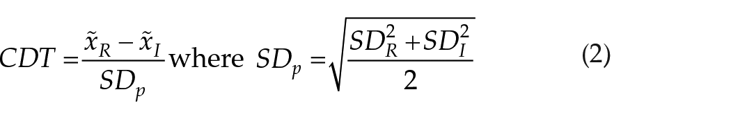
Unlike predictive accuracy metrics, statistical distance metrics such as Cohen’s Distance Test (CDT²²) and $ϕ$ -divergence measure the distance between the actual $(p)$ and imputed $(q)$ probability densities.^23,24 The CDT is defined in equation (2) where $\tilde{x}$ and $S D$ are the mean and standard deviations of the actual and imputed distributions. Distributions with small, medium, and large differences have a CDT ⩽ 0.2, 0.2 < CDT ⩽ 0.5, and 0.5 < CDT ⩽ 0.8, respectively. $ϕ$ -divergence metrics estimate the difference between $p$ and $q$ using

$D_{ϕ} (p | | q) = \int^{} p (x) ϕ (\frac{q (x)}{p (x)}) d x$

where $ϕ$ is a class of distance functions. Examples of $ϕ$ are the Kullback–Leibler (KL) divergence,²⁵ KL approximate lower-bound estimator,²⁶ and Jensen–Shannon Distance (JSDist²⁷). JSDist is defined in equation (3). A JSDist = 0 indicates identical distributions while JSDist = 1 represents maximally different distributions.

Descriptive statistics describe the characteristics of the distribution such as frequency, central tendency (mean, median, and mode), measures of variability (standard deviation and skewness), and position (quantile ranks). Normal distributions are described using mean and standard deviation. Non-normal distributions are described using median $(\tilde{X})$ , interquartile range (IQR; $r$ ), and skewness $(γ)$ . The median data point splits the distribution in half. The IQR measures the spread of the dataset and is the difference between the upper (Q3) and the lower (Q1) quartiles. Skewness measures the degree and direction of asymmetry in the dataset. A symmetrical distribution (e.g. normal distribution), left-, and right-skewed distribution has a zero, negative, and positive skewness value, respectively.

$R M S E = \sqrt{\frac{\sum_{k = 0}^{K} {(x_{I, k} - x_{R, k})}^{2}}{K}}$ (1)

$C D T = \frac{{\tilde{x}}_{R} - {\tilde{x}}_{I}}{S D_{p}} where S D_{p} = \sqrt{\frac{S D_{R}^{2} + S D_{I}^{2}}{2}}$ (2)

$\begin{matrix} J S D i s t = \sqrt{\frac{K L (p, r)}{2} + \frac{K L (q, r)}{2}} where K L (a, b) \\ = \sum_{i = 0}^{a_{b i n s}} a_{i} \times \log_{2} (\frac{a_{i}}{b_{i}}), r = \frac{p + q}{2} \end{matrix}$ (3)

Existing proposals (MIDAS,¹³ GAIN,⁴ and VAE³) assessed the deep learning imputation models using the methodology proposed in Marshall et al.²¹ with RMSE as the evaluation metric. However, the goal of imputation in the statistical literature is to capture the underlying dataset properties (e.g. mean and distribution) that are hidden by missing data to prevent bias in the subsequent analysis.^7,14 The qualitative, predictive accuracy, statistical distance, and descriptive statistics metrics evaluate different qualities of the imputation model’s performance. RMSE and CDT compare mean reconstruction, $ϕ$ -divergence metrics examine the divergence between distributions, and descriptive statistics describe distribution characteristics (e.g. median, skewness, and IQR). As a result, previous studies that have evaluated deep learning imputation using predictive accuracy metrics^4,13 may not capture the overall performance of their models. Furthermore, the aggregate RMSE is a predictive accuracy metric that may not represent the imputation model’s performance for a feature of interest $f$ . There is a need to evaluate deep learning imputation models based on the distribution of target features, reconstruction properties of interest, and the proportion of missing data.

Proposed evaluation methodology

To address the limitations in the existing imputation evaluation methodology,²¹ our proposed methodology needs to attend to the following requirements:

Requirement 1 (R1): Evaluate multiple properties of the imputation model’s reconstruction performance (e.g. mean and distribution).

Requirement 2 (R2): Summarize the imputation model’s overall reconstruction performance across multiple properties using one metric.

Requirement 3 (R3): Evaluate the trade-offs between reconstruction properties.

To address R1, we evaluate the imputation model’s performance on three metrics: (1) median, (2) skewness, and (3) IQR reconstruction. Median, skewness, and IQR were selected for this study because we are interested in imputing non-normal distributions. To address R2, we want to aggregate the median, skewness, and IQR performance. However, we cannot sum median, skewness, and IQR because each metric has different ranges and definitions. For example, a negative skew value represents a left-skewed distribution while a negative median represents a number in the dataset. To summarize the performance of multiple metrics, we need to do the following: (1) make all metric values positive, (2) compare the differences between the metric values for the imputed and target distributions instead of the values themselves, and (3) normalize each metric. Our proposed metric, reconstruction loss (RL), aggregates performance using the following equation

$R L = {\begin{array}{l} \begin{array}{l} w_{X ̃} \frac{{|a}_{q} - a_{p} |}{\max {(a}_{q}, a_{p})} + w_{γ} \frac{| b_{q} - b_{p} |}{\max (b_{q}, b_{p})} \\ + w_{r} \frac{{|c}_{q} - c_{p} |}{\max (c_{q}, c_{p})} \end{array} & if r_{q} > 0 \\ 1 & otherwise \end{array}$ (4)

where $p = actual distribution, q = imputed distribution,$

$\begin{array}{l} \tilde{X} = median, r = IQR, γ = skewness, \\ a_{q} = {\tilde{X}}_{q} + | \min {(\tilde{X}}_{q} {, \tilde{X}}_{p}) |, a_{p} = {\tilde{X}}_{p} + | \min {(\tilde{X}}_{q} {, \tilde{X}}_{p}) |, \\ b_{q} = γ_{q} + | \min (γ_{q}, γ_{p}) |, b_{p} = γ_{p} + | \min (γ_{q}, γ_{p}) |, \\ c_{q} = r_{q} + | \min (r_{q}, r_{p}) |, c_{p} = r_{p} + | \min (r_{q}, r_{p}) |, \\ w_{\tilde{X}} \in {0, 0.2, 0.4, 0.6, 0.8, 1}, w_{γ} \in {0, 0.2, 0.4, 0.6, 0.8, 1}, and \\ w_{r} \in {0, 0.2, 0.4, 0.6, 0.8, 1} \\ such that the weights satisfy the condition \\ w_{\tilde{X}} + w_{γ} + w_{r} = 1 \end{array}$ (5)

We are using weights $w_{\tilde{X}}, w_{γ}, and w_{r}$ to allow the trade-offs between the reconstruction properties to be investigated (R3). For example, in our DSS, we prefer to under-estimate effective dose (ED) exposure for safety so we assign higher weighting for median and skewness $(w_{\tilde{X}} = w_{γ} = 0.4)$ reconstruction compared to IQR $(w_{r} = 0.2)$ . Similar to hyperparameter grid searches, we consider a subset of weight tuple combinations (e.g. (1,0,0), (0.8,0.2,0), (0.6, 0.2, 0.2)) where each weight goes between 0 (not important to reconstruction performance) to 1 (most important to imputation performance) by a step set size of 0.2.^28,29 Unlike hyperparameter grid searches, we restrict the tuple combinations to sum to one (equation (5)) to evaluate the trade-offs between the metrics. Since values of all three target and model metrics can be negative, for equation (4), we need to adjust the sign of the three metrics before computing RL. Note that we are interested in the difference between the model and target distribution metrics, not each metric’s absolute value. Therefore, to make all metric values positive, we add the absolute value of the smallest number of each pair (model, target) to the three metrics: median, skewness, and IQR, when either the model or target values for each metric are negative. A RL = 0 and RL = 1 represents the best and worst reconstruction performance, respectively.

Figure 1 extends the existing imputation evaluation methodology with our proposed RL metric. First, we impute the missing data introduced into the dataset using the candidate imputation models. Second, we calculate the dataset properties (mean, skewness, and IQR) for the target and imputed distributions and perform data shifting to remove negative values, if necessary. Third, we calculate and plot the average RL metric, and the model with the best average RL value for the missing data rate is used for imputation. We can also do a parameter sweep of $w_{\tilde{X}}, w_{γ}, and w_{r}$ values to investigate the trade-offs between the imputation model’s median, skewness, and IQR reconstruction performances.

Figure 1.

Proposed imputation evaluation methodology.

Results

In this section, we present the comparative analysis of qualitative, predictive accuracy, statistical distance, descriptive statistics, and our proposed RL metric to assess two deep learning imputation models (MIDAS and GAIN) and a regression-based imputation model (PMM) on two tabular datasets. MIDAS and GAIN represent non-generative and generative deep learning imputation models, respectively. We selected PMM as our benchmark model from the statistical literature when evaluating the deep learning models’ performance.

Data collection and processing

We evaluated the imputation models (PMM, MIDAS, and GAIN) on two tabular datasets: (1) MI and (2) Credit.³⁰ The MI dataset was collected in a retrospective study we performed of all medical scans from 1200 patients who received at least one low-dose MI scan (e.g. CT and XR) from four hospitals in Canada between May 2006 and May 2017. The patients were a stratified random sample representative of the target population in terms of gender, age of first scan, and body part scanned. The patients also had above-average cumulative ED³¹ exposure. ED is a metric to estimate the uniform whole-body dose that has the same nominal radiation risk compared to the non-uniform exposure from MI.³¹ Table 2 describes the characteristics of the MI dataset. Each patient’s medical history contains demographic, health, and imaging records. Demographic data include the patient’s age, sex, year, and month of the medical visit. Health records include diagnostic codes in the International Statistical Classiﬁcation of Diseases and Related Health Problems (ICD-10-CA) format. Imaging records consist of modality (CT or XR) and body part scan (e.g. head) in the DICOM format. The ED exposure from MI is estimated using the methodology from Boursalie et al.¹² All continuous features are normalized using min–max normalization. Our study was approved by the Hamilton Integrated Research Ethics Board.

Table 2.

Medical imaging and Credit dataset characteristics.

Dataset	Instances	Years	Target (range)	Features	Range
Medical Imaging	2565 (4 hospitals, 1200 patients)	May 2006–May 2007	Effective dose (C, 1.22–43.6 mSv)	1. Age of ﬁrst scan (C)	1–91 years
				2. Year of scan (C)	2008–2016
				3. Month of scan (C)	Jan (1) to Dec (12)
				4. Sex (D)	0 (male), 1 (female)
				5–26. ICD-10 Chapters 1–21 diagnostic history (D)	0 (no previous diagnosis), 1 (previous diagnosis)
				27–48. Months since last ICD-10 Chapters 1–21 diagnosis (C)	0–96
Credit³⁰	29,206 (1 bank, 29,206 clients)	April 2005 to September 2005	Age (C, 21–79 years)	1. Sex (D)	0 (male), 1 (female)
				2. Credit limit (C)	NT$10,000–$100,000
				3–6. Education (D): High school/university/graduate/other	0 (no), 1 (yes)
				7–10. Marital status (D): Single/married/divorced/other	0 (no), 1 (yes)
				Bills (2005):
				11. April (C)	- NT$165,480 to $964,511
				12. May (C)	- NT$69,777 to $983,931
				13. June (C)	- NT$157,264 to $1.6M
				14. July (C)	- NT$170,000 to $891,586
				15. Aug (C)	- NT$81,334 to $927,171
				16. September (C)	- NT$339,603 to $961,664
				Payments (2005):
				17. April (C)	NT$0–$873,552
				18. May (C)	NT$0–$1,684,259
				19. June (C)	NT$0–$896,040
				20. July (C)	NT$0–$621,000
				21. Aug (C)	NT$0–$426,529
				22. September (C)	NT$0–$528,666
				23–28. April–September 2005 payment delay? (D)	0 (no), 1 (yes)

C: continuous and D: discrete features.

The Credit dataset³⁰ contains 30,000 banking records from clients at a Taiwanese bank between April and September 2005. Table 2 describes the characteristics of 29,206 clients who received or paid a bill between April and September 2005. Each client’s banking information includes the client’s sex, credit limit, education level, marital status, monthly bills, payments, and repayment status (bill paid on time or the amount of months payment was late). All continuous features are normalized using min–max normalization. Additional information on the Credit dataset is available at Yeh and Lien.³⁰

The MI and Credit datasets were selected for this study because they have continuous and discrete features with no missing data. The Credit dataset was also used to evaluate GAIN.⁴ Unlike previous studies,^4,13 to be consistent with the evaluation methodology,²¹ we selected one target feature for each dataset to impute. We imputed ED $f_{M I, E D}$ (MI) and age $f_{C r, A}$ (Credit). We selected ED and age for imputation because they are continuous features with non-normal distributions. There is also a relationship between the target and the remaining features to build the imputation model. For example, the ED exposure is related to the scan year as older scanners had higher exposure rates.

$f_{M I, E D}$ and $f_{C r, A}$ had non-normal distributions. As a result, we evaluated the imputation models using the original and quantile transform (QT³²) as a preprocessing step. QT maps each quantile of the non-normal feature distribution to the corresponding quantile of the normal distribution.³³ Using QT, target features with non-normal distributions can be analyzed using statistical tests (e.g. parametric) and machine learning models (e.g. Gaussian Naive Bayes) that require normal feature distributions. Machine learning models that do not require target features with normal distributions have also shown improved performance using QT features.³⁴

Evaluation procedure

We assessed the performance of PMM, MIDAS, and GAIN to impute missing data in the MI and Credit datasets. We introduced increasing proportions of data MCAR (2%, 4%, 8%, 10%, 20%, 40%, and 80%) in the target features (Table 2) after preprocessing. We validated (Supplemental Appendix A) that our missing data mechanism (MCAR) did not change the statistical properties of the train and test sets, so no data leakage (bias) occurred by preprocessing our dataset before introducing missing data. We selected the data proportions of MCAR to be consistent with previous studies.^4,13,21 We imputed the missing data at each proportion using PMM, MIDAS, and GAIN. We took the mean results $(m = 5)$ from the multiple imputation models (MIDAS and PMM) to compare performance with GAIN. Previous studies¹⁴ have demonstrated that the imputation results do not significantly change when $m > 5$ . We then repeated the evaluation five times. Each time we removed data randomly. We investigated the imputation models performances using the imputation evaluation methodology proposed in Marshall et al.²¹ with the following evaluation metrics: Histogram (benchmark), RMSE, CDT, JSDist, Median, Skewness, and IQR. We also investigated the imputation models’ performances using our proposed evaluation methodology (Figure 1) and RL metric. The histogram results were ranked based on a visual inspection of the mean and distribution reconstruction across all runs. The RMSE, CDT, JSDist, Median, Skewness, IQR, and RL results were ranked based on a visual inspection of the mean and standard deviations across all runs. The evaluation metrics represent qualitative (histogram), predictive accuracy (RMSE), statistical distance (CDT and JSDist), descriptive (median, skewness, IQR), and our aggregated RL metric. We plotted the qualitative performance (histogram) for each run. In addition, we plotted the average RMSE, CDT, JSDist, median, skewness, IQR, and RL performance over the five runs.

All experiments were conducted on a 64-bit Windows 7 laptop with a 2.8 GHz Intel Xeon CPU and 16 GB RAM. The default PMM⁵ architecture (50 epochs) was implemented using the open-source code. For MIDAS¹³ and GAIN,⁴ the default architectures (TensorFlow), loss functions (RMSE and cross-entropy), epochs (MIDAS: 20, GAIN: 10,000), optimizers (MIDAS and GAIN: Adam Optimizer), and learning rates (MIDAS: 1, GAIN: 1.5) were implemented using their open-source codes. Interested readers are referred to Lall and Robinson¹³ and Yoon et al.⁴ for full implementation details for MIDAS and GAIN, respectively.

Comparative analysis

Figure 2 shows a subset of the qualitative histogram results. $f_{M I, E D}$ and $f_{C r, A}$ had non-normal distributions. The No-QT-PMM, No-QT-MIDAS, and No-QT-GAIN models did not capture the distribution of $f_{M I, E D}$ and $f_{C r, A}$ . The imputed values from the non-generative models (PMM and MIDAS) had a more normal distribution centered on the average value of the target features. On the contrary, the generative model (GAIN) suffered from mode collapse.⁴ Mode collapse occurs when the GAIN discriminator does not distinguish well between the actual and imputed data. As a result, the GAIN generator learns to fool the discriminator by generating modes of data that are not representative of the feature distribution. Our results show that PMM and MIDAS had improved performance when $f_{M I, E D}$ and $f_{C r, A}$ were represented using a QT. For PMM and MIDAS, the imputation models better captured the distributions of $f_{M I, E D}$ and $f_{C r, A}$ . The QT-GAIN models did not capture the mode or distribution of the data.

Figure 2.

Histogram of $f_{M I, E D}$ (top; bin width = 2 mSv) and $f_{C r, A}$ (bottom; bin width = 2 years) imputation at 2% and 80% missing data over two runs (rows). (A color version of this figure is available in the online journal.)

The imputation models’ RMSE performances imputing $f_{M I, E D}$ are shown in Figure 3(a). The No-QT-MIDAS and QT-MIDAS model had the best and second-best RMSE performance across all missing data rates, respectively. The No-QT-PMM and QT-PMM models performed third best overall. The No-QT-GAIN model had similar performance to the MIDAS and PMM models for 2–40% missing rates. However, the No-QT-GAIN model’s mode collapse was poorly detected using RMSE. The No-QT-GAIN models captured the $f_{M I, E D}$ mean (Figure 2), which minimized their RMSE. The QT-GAIN model captured the maximum $f_{M I, E D}$ values, which resulted in the worst RMSE performance. The imputation models’ RMSE performances were consistent on the Credit imputation (Figure 3(b)) except for the No-QT-MIDAS, QT-MIDAS, and QT-PMM models, which all had similar performances. Interestingly, the imputation models’ RMSE performances did not agree with the qualitative results (Figure 2). In addition, the improved distributional performance of the QT models was not captured using RMSE.

Figure 3.

RMSE (a and b), CDT (c and d), and JSDist (e and f) evaluation results for $f_{M I, E D}$ (left) and $f_{C r, A}$ (right) at increasing missing data rates. Lines and error bars are average performance over ﬁve runs. (A color version of this figure is available in the online journal.)

Figure 3(c) shows the CDT performances for the $f_{M I, E D}$ imputation models. The No-QT-MIDAS, No-QT-PMM, and QT-PMM models had the best CDT performances. Next, the QT-MIDAS had the second-best CDT performance. Then, the No-QT-GAIN and QT-GAIN models had the worst CDT performance. Similar to RMSE, the GAIN model’s mode collapse was poorly detected using CDT. CDT compares the mean and standard deviations of the actual and imputed data (equation (2)). As a result, the GAIN models had competitive and stable CDT performance despite not capturing the $f_{M I, E D}$ distribution. The $f_{C r, A}$ imputation had similar CDT performance (Figure 3(d)) across all models. The $f_{C r, A}$ GAIN imputation models also had the most unstable CDT results. Like RMSE, the CDT results for both datasets did not agree with the qualitative results (Figure 2). The improved distributional performance of the QT imputation models was also not captured using CDT.

The imputation models’ JSDist performances imputing $f_{M I, E D}$ are shown in Figure 3(e). The No-QT-PMM and QT-PMM models had the best JSDist performance for $f_{M I, E D}$ imputation. Next, the QT-MIDAS model had the second-best JSDist performance. Then, the No-QT-MIDAS, No-QT-GAIN, and QT-GAIN models had the worst and most unstable JSDist performance. Unlike RMSE and CDT, the JSDist metric detected mode collapse in the GAIN models. The GAIN model’s capture of the mean $f_{M I, E D}$ values did not achieve competitive JSDist performance. On the Credit dataset (Figure 3(f)), the QT-PMM model had the best JSDist performance while the No-QT-PMM model performed second best. The No-QT-MIDAS, QT-MIDAS, and QT-GAIN models had the worst JSDist performance. Unlike the predictive accuracy metrics, the JSDist metrics for the $f_{M I, E D}$ and $f_{C r, A}$ imputation models agreed with the qualitative results. JSDist is a quantitative implementation of the qualitative comparison (Figure 2), so the agreement between the evaluation metrics is understandable. The improved distributional performance of the QT models was also captured by the JSDist metric.

The median metric results of the $f_{M I, E D}$ imputation models are shown in Figure 4(a). The QT-MIDAS and QT-PMM models had the best and second-best median reconstruction for $f_{M I, E D}$ , respectively. The No-QT-MIDAS, No-QT-PMM, and GAIN models had the worst median reconstruction performances. The GAIN models’ performance was also the most unstable as mode collapse enabled the models to achieve competitive performance in some runs. However, the median metric was unable to identify mode collapse in the GAIN models. On the Credit dataset (Figure 4(b)), the No-QT-PMM, QT-PMM, QT-MIDAS, and No-QT-MIDAS models had similar median reconstruction performance. The No-QT-GAIN and QT-GAIN models had the worst performance on the credit dataset.

Figure 4.

Median (a and b), skewness (c and d), and IQR (e and f) descriptive statistics results for $f_{M I, E D}$ (left) and $f_{C r, A}$ (right) at increasing missing data rates. Lines and error bars are average performance over ﬁve runs. (A color version of this figure is available in the online journal.)

The skewness metric results of the $f_{M I, E D}$ imputation models are shown in Figure 4(c). The QT-MIDAS model had the best skewness reconstruction for $f_{M I, E D} .$ The No-QT-PMM and QT-PMM models had the second-best skewness performances. The No-QT-MIDAS, No-QT-GAIN, and QT-GAIN models had the worst skewness performances. The mode collapse also resulted in poor and unstable skewness reconstruction performance for the No-QT-GAIN and QT-GAIN models. On the Credit dataset (Figure 4(d)), the No-QT-PMM, QT-PMM, No-QT-MIDAS, and QT-MIDAS models had similar skewness reconstruction performances. The No-QT-GAIN and QT-GAIN models had the worst performances on the Credit dataset.

The IQR metric results of the $f_{M I, E D}$ imputation models are shown in Figure 4(e). The No-QT-MIDAS model had the best IQR reconstruction for $f_{M I, E D}$ . Interestingly, the remaining models (QT-MIDAS, No-QT-PMM, QT-PMM, No-QT-GAIN, and QT-GAIN) all failed to capture the IQR reconstruction. The poor IQR reconstruction performance was not captured by the predictive accuracy and statistical distance metrics. On the credit dataset (Figure 4(f)), the No-QT-MIDAS and QT-MIDAS models had the best IQR reconstruction performance, and the No-QT-PMM and QT-PMM models performed second best. The No-QT-GAIN and QT-GAIN models had the worst performance on the credit dataset.

Figure 5 shows a subset of the average RL performance for the $f_{M I, E D}$ imputation models for 80% missing data over five runs. Overall, QT-MIDAS (Figures 5(a) and 6(a)) and QT-PMM models (Figures 5(c) and 6(c)) achieved the highest RL performance over the entire range of $w_{\tilde{X}}, w_{γ}, and w_{r}$ values for $f_{M I, E D}$ imputation. No-QT-PMM (Figures 5(d) and 6(d)) had the second-best RL performance across all weight combinations. No-QT-MIDAS (Figures 5(b) and 6(b)), No-QT-GAIN (Figures 5(e) and (f)), and QT-GAIN (Figure 6(e) and (f)) models had the worst RL performance. No-QT-MIDAS poor RL performance captures the model’s poor mean and skewness reconstruction performance. Similarly, the poor RL performances for the No-QT-GAIN and QT-GAIN models capture the model’s mode collapse. On the Credit dataset (Figure 6), the No-QT-MIDAS and QT-MIDAS models had the best performance while the No-QT-PMM and QT-PMM models had the second-best performance. The RL metric shows the trade-off between improved median and skewness reconstruction (MIDAS) and IQR reconstruction (PMM models). The No-QT-GAIN and QT-GAIN mode collapse was also captured by the RL metric.

Figure 5.

RL values for QT MIDAS (a), No-QT MIDAS (b), QT PMM (c), No-QT PMM (d), QT GAIN (e), and No-QT GAIN (f) imputation models for 80% missing $f_{M I, E D}$ data. The axes show the $w_{X ̃}, w_{γ}, and w_{r}$ values. The color of each circle shows the average RL value for the $w_{X ̃}, w_{γ}, and w_{r}$ combination (RL = 0 and RL = 1 represents best and worst reconstructive performance, respectively). (A color version of this figure is available in the online journal.)

Figure 6.

RL values for QT MIDAS (a), No-QT MIDAS (b), QT PMM (c), No-QT PMM (d), QT GAIN (e), and No-QT GAIN (f) imputation models for 80% missing $f_{C r, A}$ data. The axes show the $w_{X ̃}, w, and w_{r}$ values. The color of each circle shows the average RL value for the $w_{X ̃}, w_{γ}, and w_{r}$ combination (RL = 0 and RL = 1 represents best and worst reconstructive performance, respectively). (A color version of this figure is available in the online journal.)

Discussion

Table 3 ranks each imputation model’s performance based on the qualitative, predictive accuracy, and statistical distance metrics for each dataset we investigated. The qualitative results were ranked based on a visual inspection of the mean and distribution reconstruction (Figure 2) across all runs. Based on the histogram (benchmark) results, the QT-PMM would be selected for imputation in both datasets across all missing data rates. However, the predictive accuracy metrics did not agree with the qualitative and statistical distance results. The No-QT-MIDAS would be selected for the MI dataset and the No-QT-PMM, No-QT-MIDAS, or QT-MIDAS models would be selected for the Credit dataset based on RMSE. Using CDT, the No-QT-PMM, QT-PMM, or No-QT-MIDAS model would be selected for the MI dataset and the No-QT-PMM, QT-PMM, No-QT-MIDAS, or QT-MIDAS would be selected for the Credit dataset. The JSDist ranking agreed with the histogram results. The qualitative results (Figure 2) provide an initial check of the imputation model’s performance⁷ and provide context to the quantitative metrics. For example, the qualitative results demonstrate that the poor performance of the GAIN models is due to mode collapse. The qualitative results can also be reviewed by an expert to evaluate imputation models with similar performance. For example, a medical expert could review the qualitative results of the No-QT-PMM and QT-PMM models (Figure 3(e)). Our results demonstrate that the predictive accuracy metrics evaluate the imputation model’s ability to capture the mean of the target distributions. For example, RMSE directly compares the imputed estimates with the actual values rather than comparing the distributions (equation (1)). Similarly, CDT compares the means and standard deviations of the imputed and actual distributions (equation (2)). Interestingly, the imputation models that generate more normal distributions (MIDAS and no-QT models) minimized their RMSE and CDT (Figure 3(a) to (d)) without capturing the distribution of the target features. In fact, the PMM models that attempted to capture the distribution of the target features (Figure 2) had poorer RMSE and CDT performance (Figure 3(a) to (d)). In addition, the GAIN models demonstrate how competitive RMSE and CDT results (Figure 3(a) to (d)) can be achieved by imputing a single value due to mode collapse. Our results demonstrate how imputation models can achieve good predictive accuracy performance (Figure 3) without capturing the feature’s distribution (Figure 2). The $ϕ$ -divergence metric (JSDist) best assessed the imputation model’s performance. Unlike predictive accuracy metrics, JSDist (equation (3)) compares the target and imputed distributions rather than comparing imputed instances directly with their actual values. In our study, the target features had a non-normal distribution. As a result, an imputation model that generates a more normal distribution (GAIN and no-QT models) will diverge from the target feature distribution (Figure 2). In addition, an imputation model that captures the mean or mode of the model (Figure 2) results in poor JSDist (Figure 3(e) to (f)) performance despite competitive RMSE and CDT (Figure 3(a) to (d)) results. Divergence metrics have been used to evaluate generative deep learning models for image generation.¹⁹ Our results demonstrate that $ϕ$ -divergence metrics can also be used to evaluate deep learning imputation models.

Table 3.

Imputation models’ ranked performances (1 best, 4 worst) based on the evaluation metrics.

	Medical imaging (ED)						Credit (age)
	PMM		MIDAS		GAIN		PMM		MIDAS		GAIN
	No-QT	QT	No-QT	QT	No-QT	QT	No-QT	QT	No-QT	QT	No-QT	QT
Histogram	1	1	3	2	3	3	1	1	2	2	3	3
RMSE	3	3	1	2	3	4	1	2	1	1	3	3
CDT	1	1	1	2	3	3	1	1	1	1	2	2
JSDist	1	1	3	2	3	3	2	1	3	3	4	4
Median	3	2	3	1	4	4	1	1	1	1	2	2
Skewness	2	2	3	1	4	4	1	1	1	1	2	2
IQR	2	2	2	1	3	3	2	2	1	1	3	3
RL	2	1	3	1	3	3	2	2	1	1	3	3

ED: effective dose; PMM: predictive mean matching; MIDAS: Multiple Imputation with Denoising Autoencoders; GAIN: Generative Adversarial Imputation Nets; QT: quantile transform; RMSE: root mean square error; CDT: Cohen’s Distance Test; IQR: interquartile range; RL: reconstruction loss.

The descriptive statistics assessed different characteristics of the imputation model’s performance (median, skewness, and IQR). Interestingly, the deep learning–based model (QT MIDAS) competitive reconstruction performance was not captured when evaluating the models using the RMSE, CDT, and JSDist metrics. Our results demonstrate that previous studies that have evaluated deep learning imputation using predictive accuracy metrics^4,13 may not capture the overall performance of their models. However, our findings also suggest that the performance metric should be selected based on the dataset size, distribution of features, and proportion of missing data. While descriptive statistic metrics provided us insights into the imputation model’s behavior on the ED dataset, the metrics were not as sensitive in evaluating imputation performance on the Credit dataset (Figure 4). Overall, our study demonstrated that qualitative, predictive accuracy, statistical distance, and descriptive statistics investigate different properties of reconstruction performance, and there is a need to aggregate performance between these metrics.

Our proposed evaluation methodology (Figure 1) successfully ranked the performance of the imputation models. Unlike the existing methodology (section “Materials and methods”), our methodology considered multiple aspects of the imputation model’s reconstruction performance (mean, skewness, and IQR). In addition, our methodology provides a mechanism for users to study the trade-offs between the reconstruction criteria. For example, the best balance between median, skewness, and IQR reconstruction was achieved by the MIDAS model. Unlike RMSE, CDT, and JSDist, our methodology did not penalize the MIDAS and PMM models for attempting to capture the distribution of the target features at the expense of mean and skewness reconstruction. Our methodology also provides a mechanism to incorporate expert opinion when selecting an imputation model beyond qualitative analysis.

In the statistical imputation literature, researchers impute datasets using multiple methods and investigate their impact on the downstream predictive model. Our proposed evaluation methodology provides researchers with a quantitative method to select the imputation models for further study. For example, we can investigate how the downstream deep learning model’s performance changes when imputing data using GAIN (mean imputation), PMM (IQR imputation), and MIDAS (median, skewness, and IQR imputation) models.

RL can be used to evaluate the imputation model’s performance on normal and non-normal target distributions. However, the dataset properties may determine the suitability of the evaluation metrics to assess the imputation models. For example, the statistical distance metric (JSDist) may better capture the difference between the target and imputed distributions for non-normal distributions compared to predictive accuracy metrics. Similar to statistical tests,⁵ the choice of metric may depend on the dataset size. In our study, the metrics had similar performances (Figures 3 to 6) between datasets with different sizes (Table 2).

Our study exhibits some limitations. First, we investigated the imputation model’s performance on specific features (ED and age). In addition, data MAR and MNAR were not investigated. Finally, we investigated the default model architectures. Improved model architecture and training could impact performance evaluation.

Related work

An important component in deep learning is evaluating performance. Previous studies have evaluated various properties of the deep learning models’ performances such as accuracy, computational,³⁵ robustness,³⁶ privacy,³⁷ ethical,³⁸ and trust.³⁹ Increasingly, deep learning models are evaluated using multiple performance metrics.³⁵ Furthermore, benchmarks⁴⁰ are being developed to evaluate new models with prior work using open-source datasets (e.g. ImageNet⁴¹). There is also a growing body of literature surveying the strengths and limitations of evaluation metrics for deep learning^19,42,43 to assist researchers and developers to select their evaluation metrics. For example, Borji^19,44 and Thompson et al.⁴³ have surveyed evaluation metrics to assess GANs image generation and graph generative model (GGM) performances, respectively. Borji^19,44 demonstrated how qualitative and quantitative evaluation metrics assessed various aspects of the deep learning model’s image generation performance. Borji recommended using multiple metrics to assess various elements of the GAN’s performance. Thompson et al.⁴³ performed a comparative analysis of evaluation metrics to rank the GGM’s fidelity, diversity, sample efficiency, and computational performance. However, the existing surveys did not investigate evaluation metrics to assess deep learning–based imputation models on heterogeneous datasets.

In statistics, there is a large body of surveys on metrics that can be used to evaluate imputation models. For example, Deza and Deza⁴⁵ encyclopedia of distances provides an overview of available distance metrics for comparing distributions. Previous studies^7,19 also provide guidelines for researchers to select their metrics to evaluate statistical imputation models. Nguyen et al.⁷ reviewed evaluation metrics (qualitative, predictive accuracy metrics, and posterior predictive checking) to assess imputation models. Like Borji, Nguyen et al. recommended using different metrics to assess various elements of imputation models.

Despite advances in the deep learning and statistical literature, existing deep learning imputation models (MIDAS,¹³ GAIN,⁴ and VAE³) have been assessed using RMSE, a predictive accuracy metric. The studies showed the deep learning imputation models had competitive RMSE performance compared to statistical imputation models. However, deep learning imputation models can impute missing data in multiple features at once. As a result, Lall and Robinson¹³ and Yoon et al.⁴ assessed the deep learning imputation model’s aggregate performance using one metric (RMSE) across all features with missing data. However, there are scenarios where specific features need to be imputed. For example, we need to impute a target feature (ED) to develop our DSS as the remaining features in our dataset are complete. The deep learning imputation model’s performance for different reconstruction properties has not been investigated. In addition, the deep learning imputation model’s performance using qualitative and quantitative metrics has not been studied. In this article, we compared two deep learning imputation models (DAE and GAN) using qualitative, predictive accuracy, and statistical distance metrics on two tabular datasets. We also proposed and evaluated extensions to the existing evaluation methodology to assess the performance of deep learning–based imputation models.

Conclusions

The existing evaluation methodology commonly used to assess deep learning–based imputation models lacks a mechanism to evaluate and investigate multiple aspects of the model’s reconstruction performance. To address this challenge, we proposed an evaluation methodology and an RL metric to assess deep learning–based imputation models. Our methodology ranks imputation models by their performance across multiple reconstruction properties such as median, skewness, and IQR. Our methodology also provides researchers with a mechanism to evaluate the trade-offs between reconstruction properties. We used our evaluation methodology to assess two deep learning imputation models on two tabular datasets. We also described the strengths and challenges of using evaluation metrics to assess deep learning–based imputation models.

Given these results, we are extending our proposed imputation evaluation methodology to rank the deep learning model’s imputation performance across multiple features with missing data. In addition, we will investigate how deep learning imputations perform for multiple features compared to statistical imputation models. Finally, we are investigating methods to improve visualizing the trade-offs between imputation performance metrics.

Supplemental Material

sj-docx-1-ebm-10.1177_15353702221121602 – Supplemental material for Evaluation methodology for deep learning imputation models

Supplemental material, sj-docx-1-ebm-10.1177_15353702221121602 for Evaluation methodology for deep learning imputation models by Omar Boursalie, Reza Samavi and Thomas E. Doyle in Experimental Biology and Medicine

Footnotes

Authors’ Contributions

All authors participated in the design,interpretation of the studies and analysis of the data,and review of the manuscript;OB wrote the manuscript.

Declaration of Conflicting Interests

The author(s) declared no potential conflicts of interest with respect to the research,authorship,and/or publication of this article.

Funding

The author(s) disclosed receipt of the following financial support for the research,authorship,and/or publication of this article: This work was supported by the Natural Sciences and Engineering Research Council of Canada,Southern Ontario Smart Computing Innovation Platform,and the Canadian Department of National Defense: Innovation for Defense Excellence & Security Program.

ORCID iD

Omar Boursalie

Supplemental Material

Supplemental material for this article is available online.

References

Rubin

DB.

Inference and missing data.

Biometrika 1976;63:581–92

Wells

Chagin

Nowacki

Kattan

MW.

Strategies for handling missing data in electronic health record derived data.

EGEMS (Wash DC) 2013;1:1035–7

Nazábal

Olmos

Ghahramani

Valera

Handling incomplete heterogeneous data using VAEs.

Pattern Recognit 2020;107:1–11

Yoon

Jordon

Schaar

GAIN: missing data imputation using generative adversarial nets. In: Proceedings of the 35th international conference on machine learning, Stockholm, 10–15 July 2018, pp.5689–98. Proceedings of Machine Learning Research (PMLR).

Buuren

Groothuis-Oudshoorn

MICE: multivariate imputation by chained equations in R.

J Stat Softw 2010;45:1–45

Pham

Tran

Phung

Venkatesh

Predicting healthcare trajectories from medical records: a deep learning approach.

J Biomed Inform 2017;69:218–29

Nguyen

Carlin

Lee

KJ.

Model checking in multiple imputation: an overview and case study.

Emerg Themes Epidemiol 2017;14:8–12

García

Luengo

Herrera

Tutorial on practical tips of the most influential data preprocessing algorithms in data mining.

Knowl Based Syst 2016;98:1–29

Boursalie

Samavi

Doyle

Koff

. Deep learning model for cancer risk from low dose medical imaging radiation. Eur Radiol 2020. DOI: 10.26044/esi2020/ESI-10315

10.

González

ABd

Mahesh

Kim

K-P

Bhargavan

Lewis

Mettler

Land

. Projected cancer risks from computed tomographic scans performed in the United States in 2007. Arch Intern Med Res 2009;169:2071–7

11.

Mathews

Forsythe

Brady

Butler

Goergen

Byrnes

Giles

Wallace

Anderson

Guiver

McGale

Cain

Dowty

Bickerstaffe

Darby

SC.

Cancer risk in 680 000 people exposed to computed tomography scans in childhood or adolescence: data linkage study of 11 million Australians.

BMJ 2013;346:1–18

12.

Boursalie

Samavi

Doyle

Koff

DA.

Using medical imaging effective dose in deep learning models: estimation and evaluation.

IEEE Trans Radiat Plasma Med Sci 2021;5:245–52

13.

Lall

Robinson

The MIDAS touch: accurate and scalable missing-data imputation with deep learning.

Polit Anal 2022;30:179–96

14.

Buuren

SV.

Flexible imputation of missing data. 1st ed. Boca Raton, FL: Chapman and Hall/CRC, 2018

15.

Boursalie

Samavi

Doyle

. Evaluation metrics for deep learning imputation models. In: Shaban-Nejad

Michalowski

Bianco

(eds) International workshop on health intelligence: AI for disease surveillance and pandemic intelligence. Cham: Springer, pp.309–22

16.

Little

Rubin

DB.

Statistical analysis with missing data. 2nd ed. Hoboken, NJ: John Wiley & Sons, 2002

17.

Rubin

DB.

Statistical matching using file concatenation with adjusted weights and multiple imputations.

J Bus Econ Stat 1986;4:87–94

18.

Voulodimos

Doulamis

Protopapadakis

Deep learning for computer vision: a brief review.

Comput Intell Neurosci 2018;2018:7068349

19.

Borji

Pros and cons of GAN evaluation measures.

Comput Vis Image Underst 2019;179:41–65

20.

Rubin

. An overview of multiple imputation. Alexandria, VA: ASA SRMS, 1988

21.

Marshall

Chahin

Rush Bea . Secondary analysis of electronic health records. 1st ed. Cham: Springer, 2016

22.

Cohen

Statistical power analysis for the behavioral sciences. 2nd ed. Mahwah, NJ: Lawrence Erlbaum Associates, 2013

23.

Nowozin

Cseke

Tomioka

f-GAN: training generative neural samplers using variational divergence minimization.

Adv Neural Inf Process Syst 2019;29:457–66

24.

Kingma

Welling

Auto-encoding variational Bayes. In: International conference on learning representations, Banff, AB, Canada, 14–16 April 2014, pp.1–14

25.

Kullback

Leibler

RA.

On information and sufficiency.

Ann Math Stat 1951;22:79–86

26.

Arbel

Zhou

Gretton

Generalized energy based models. In: International conference on learning representations, Virtual Event, 3–7 May 2021, pp.1–36

27.

Briët

Harremoës

Properties of classical and quantum Jensen-Shannon divergence.

Phys Rev A 2009;79:1–11

28.

Fridovich-Keil

Recht

. Choosing the step size: intuitive line search algorithms with efficient convergence. In: 11th annual workshop on optimization for machine learning, Vancouver, BC, Canada, 14 December 2019, pp.1–21. Curran Associates.

29.

Falkowski

Nicholls

MG.

Increasing the efficiency of selected grid search procedures through the introduction of a best step mechanism.

J Heuristics 1999;5:199–214

30.

Yeh

Lien

C-h.

The comparisons of data mining techniques for the predictive accuracy of probability of default of credit card clients.

Expert Syst Appl 2009;36:2473–80

31.

ICRP. The 2007 recommendations of the International Commission on Radiological Protection (ICRP) Publication 103. Ann ICRP 2007;37:1–332

32.

Pedregosa

Varoquaux

Gramfort

Michel

Thirion

Grisel

Blondel

Prettenhofer

Weiss

Dubourg

Vanderplas

Passos

Cournapeau

Brucher

Perrot

Duchesnay

É.

Scikit-learn: machine learning in Python.

J Mach Learn Res 2011;12:2825–30

33.

Beasley

Erickson

Allison

DB.

Rank-based inverse normal transformations are increasingly used, but are they merited.

Behav Genet 2009;39:580–95

34.

Song

Yang

K-means clustering of overweight and obese population using QT metabolic data.

Diabetes Metab Syndr Obes 2019; 12:1573–82

35.

Boursalie

Samavi

Doyle

TE.

Machine learning and mobile health monitoring platforms: a case study on research and implementation challenges.

J Healthc Inform Res 2018;2:179–203

36.

Bastani

Ioannou

Lampropoulos

Vytiniotis

Nori

Criminisi

Measuring neural net robustness with constraints. In: NIPS’16: Proceedings of the 30th international conference on neural information processing systems, Barcelona, 5–10 December 2016, pp.1–9. Red Hook, NY: Curran Associates

37.

Liu

Ding

Shaham

Rahayu

Farokhi

Lin

When machine learning meets privacy.

ACM Comput Surv 2021;54:1–36

38.

Safdar

Banja

Meltzer

CC.

Ethical considerations in artificial intelligence.

Eur J Radiol 2020;122:108768

39.

Thomas

Samavi

Doyle

. Trust quantification for autonomous medical advisory systems. In: 2021 18th international conference on privacy, security and trust (PST), Auckland, New Zealand, 13–15 December 2021, pp.1–7, New York: IEEE

40.

Zhang

Zha

Lin

Liang

A survey on deep learning benchmarks: do we still need new ones? In: Zheng

Zhan

(eds) Benchmarking, measuring, and optimizing. Cham: Springer, 2019, pp.36–49

41.

Deng

Dong

Socher

Kai

F-F.

ImageNet: a large-scale hierarchical image database. In: 2009 IEEE conference on computer vision and pattern recognition, Miami, FL, 20–25 June 2009, pp.248–55. New York: IEEE

42.

Nayyer

Ajmal

Wei

Zulqarnain

Mubarak

Video description: a survey of methods, datasets, and evaluation metrics.

ACM Comput Surv 2019;52:1–37

43.

Thompson

Knyazev

Ghalebi

Kim

Taylor

. On evaluation metrics for graph generative models. In: International conference on learning representations, Virtual Event, 25–29 April 2022, pp.1–30

44.

Borji

Pros and cons of GAN evaluation measures: new developments.

Comput Vis Image Underst 2022;215:1–35

45.

Deza

Encyclopedia of distances. 2nd ed. Cham: Springer, 2009

Supplementary Material

Please find the following supplemental material available below.

For Open Access articles published under a Creative Commons License, all supplemental material carries the same license as the article it is associated with.

For non-Open Access articles published, all supplemental material carries a non-exclusive license, and permission requests for re-use of supplemental material or any part of supplemental material shall be sent directly to the copyright owner as specified in the copyright notice associated with the article.

0.02 MB

0.00 MB