A new algorithm for considering green communication and excellent sensing performance in cognitive radio networks

Abstract

Multi-node cooperative sensing can effectively improve the performance of spectrum sensing. Multi-node cooperation will generate a large number of local data, and each node will send its own sensing data to the fusion center. The fusion center will fuse the local sensing results and make a global decision. Therefore, the more nodes, the more data, when the number of nodes is large, the global decision will be delayed. In order to achieve the real-time spectrum sensing, the fusion center needs to quickly fuse the data of each node. In this article, a fast algorithm of big data fusion is proposed to improve the real-time performance of the global decision. The algorithm improves the computing speed by reducing repeated computation. The reinforcement learning mechanism is used to mark the processed data. When the same environment parameter appears, the fusion center can directly call the nodes under the parameter environment, without having to conduct the sensing operation again. This greatly reduces the amount of data processed and improves the data processing efficiency of the fusion center. Experimental results show that the algorithm in this article can reduce the computation time while improving the sensing performance.

Introduction

Developments in wireless communication technology have increased the need for spectrum resources, which are currently limited.^1,2 To address this problem, cognitive radio networks have been proposed to improve existing spectrum resources.^3,4 In this context, spectrum sensing technology is the basic link between cognitive radio networks. ⁵

Sensing nodes need to quickly and accurately perform spectrum sensing in order to efficiently utilize the idle frequency band without interfering with the primary user. ⁶ This presents another issue; due to the impacts of path loss, shadow fading, and hidden terminals, it is difficult for a single sensor node to accurately detect the primary user’s status.^7,8 Nevertheless, cooperative sensing can effectively overcome these impacts by fusing detection information from multiple nodes in different geographical locations. ⁹ In centralized cooperative sensing, there is a special data fusion center in the cognitive network. This collects local perception results from the nodes participating in cooperative perception, judges the current usage of authorized bands, and then broadcasts the decision results in the network or directly controls and schedules the perception nodes. ¹⁰ The local sensing result collection process will increase the communication overhead when a large number of nodes are participating.^11,12 However, too many cooperative cognitive users (sensing nodes) will cause vast communication overhead. A proposed review method addressed this problem by examining the observed values of perceived nodes and only allowing nodes containing sufficient information to send their decision values (0 or 1) to the fusion center. ¹³ This method reduces communication overhead but also reduces sensing performance. Aiming at the excessive overhead created by equal gain fusion,^14,15 a double threshold method is used to perform cooperative spectrum sensing in which each node adopts double threshold detection and sends the detected value directly to the fusion center, which then makes the judgment. Combined with the judgments of each node and its own judgment, the fusion center makes two judgments to determine whether the primary user exists. This employs a combination of soft and hard fusion methods, but performs two operations in the fusion center, thus increasing computational power. Furthermore, a hierarchical cooperative spectrum detection method has been proposed to solve the problem of excessive cooperative sensing overhead.^16,17 Here, when nodal observation values are between two thresholds, the region between these two thresholds is evenly divided into four parts; four different regions are thus quantized by 2 bits. The sensing nodes then send 2 bits of information to the fusion center. When compared with the equal gain fusion method, this reduces communication overhead. However, the sensing performance of hard fusion decreases. ¹⁸

Spectrum sensing performance directly affects the throughput of cognitive users, ¹⁹ and multi-node cooperative spectrum sensing is a common method to improve the performance of spectrum sensing. ²⁰ However, when multi-node participates in cooperative sensing, the sensing data will increase greatly, and the fusion center cannot process a large number of data in time, which will cause delayed decision, which will affect the security of the main user or the throughput of cognitive users. In order to make a decision in time, a large number of data in the fusion center needs to be processed quickly, which requires the selection of some node data to reduce the number of processed data. Therefore, in order to achieve the real-time spectrum sensing, the fusion center needs to quickly fuse the data of each node. In this article, a fast algorithm of big data fusion is proposed to improve the real-time performance of the global decision. The algorithm improves the computing speed by reducing repeated computation. The reinforcement learning mechanism is used to mark the processed data. When the same environment parameter appears, the fusion center can directly call the nodes under the parameter environment, without having to conduct the sensing operation again. This greatly reduces the amount of data processed and improves the data processing efficiency of the fusion center. Experimental results show that the algorithm in this article can reduce the computation time while improving the perceived performance.

System model

This study designed an analog cognitive radio system consisting of a primary user (PU) and 16 nodes (cognitive users). ²¹ Each node communicates with the fusion center through a channel, while the fusion center fuses information from each node to determine whether the primary user channel is idle. The system model is illustrated in Figure 1.

Figure 1.

Simulation scenario for spectrum sensing.

Derivation of the optimum local detection threshold

For spectrum sensing, every SU independently performs an energy detection process. The signal received by an SU is determined as follows ²²

$$x(m)=\mathrm{hs}(m)+v(m),m=0,1,\dots ,M-1$$ (1)

where $s(m)$ is a PU signal, $v(m)$ is the additive white Gaussian noise with zero mean and variance ${\sigma }_v^2$ , $m$ represents the serial number of the sampling point, $M$ is the number of samples, and h is channel gain. Suppose PU is absent (i.e. $s(m)=0$ ); the hypothesis of free channel is then denoted by $H_0$ , whereas the hypothesis of busy channel is denoted by $H_1$ , as follows ²³

$$\begin{array}{c}{H}_0:x(m)=v(m),m=0,1,\dots ,M-1\hfill \\ H_1:x(m)=\mathrm{hs}(m)+v(m),m=0,1,\dots ,M-1\hfill \end{array}$$ (2)

Assuming E is the average collected energy of an SU and it is expressed as follows ²⁴

$$E=\frac{1}{M}\sum _{m=0}^{M-1}{|x(m)|}^2$$ (3)

If each SU can make its local decision according to single threshold ${\lambda }_o$ with probabilities of detection $P_d$ and false alarm $P_f$ , the equation is as follows ²⁵

$$P_d=P\{E\ge {\lambda }_o|H_1\}=Q\left(\frac{{\lambda }_o-({\sigma }_s^2+{\sigma }_v^2)}{({\sigma }_s^2+{\sigma }_v^2)/\sqrt{M/2}}\right)$$ (4)

$$P_f=P\{E\ge {\lambda }_o|H_0\}=Q\left(\frac{{\lambda }_o-{\sigma }_v^2}{{\sigma }_v^2/\sqrt{M/2}}\right)$$ (5)

where ${\sigma }_s^2$ is signal power and ${\sigma }_v^2$ is noise power; the complementary cumulative distribution function $Q(x)$ will be described as follows ²⁶

$$Q\left(x\right)=\frac{1}{\sqrt{2\pi }}\underset{x}{\overset{\infty }{\int }}{e}^{\frac{-t^2}{2}}\mathrm{dt}$$ (6)

Assuming the presence probability of a PU is $P(H_1)=\beta$ , $0<\beta <1$ and the absence probability of the PU is $P(H_0)=1-\beta$ , then the probability of error detection ( $P_e$ ) is as follows ²⁷

$$P_e=P\left(H_1\right)(1-P_d)+P\left(H_0\right)P_f=\beta (1-P_d)+(1-\beta )P_f$$ (7)

where $P_e$ is the quadratic function of the ${\lambda }_o$ , we can derive ${\partial }^2{P}_e/{\partial }^2{\lambda }_o>0$ . The optimal threshold ${\lambda }_o$ is obtained by $\partial P_e/\partial {\lambda }_0=0$ and it is expressed as follows ²⁸

$${\lambda }_o=\frac{{\sigma }_v^2(1+\gamma )[1+\sqrt{1+\frac{4(2+\gamma )}{M·\gamma }\ln \left[\frac{(1-\beta )(1+\gamma )}{\beta }\right]}]}{2+\gamma }$$ (8)

It is easy to obtain optimal threshold ${\lambda }_o$ if signal power ${\sigma }_s^2$ , noise power ${\sigma }_v^2$ and the SNR of the SU’s receiving terminal are known.

Estimating the optimal threshold

If a sensing cycle sampling point is $M=2^L$ and L is a positive integer, M can be divided into the two following equal sections: (1) the previous $M/2$ sampling points can be expressed with $x_1$ ; (2) the later $M/2$ sampling points can be expressed with $x_2$ . $x_1$ and $x_2$ are given as follows

$$x_1=(x\left(0\right),x\left(1\right),\dots ,x(M_1-1))$$ (9)

$$x_2=(x\left(M_1\right),x(M_1+1),\dots ,x(M-1))$$ (10)

where $M_1=M/2$ , the average energy of each section is expressed as follows

$$E_1=\frac{1}{M_1}\sum _{m=0}^{M_1-1}{\left|x\left(m\right)\right|}^2$$ (11)

$$E_2=\frac{1}{M_1}\sum _{m=M_1}^{M-1}{\left|x\left(m\right)\right|}^2$$ (12)

If $E_1<E_2$ , $x_1$ denotes AWGN, $x_2$ denotes the sum of signal and AWGN (i.e. $E_1={\sigma }_v^2$ ), $E_2={\sigma }_v^2+{\sigma }_s^2$ . If $E_1>E_2$ , $x_2$ denotes AWGN.

Let $E_1$ denote estimated noise power ${\hat{\sigma }}_v^2$ and $E_2$ denote the estimated sum of signal and noise powers ${\hat{\sigma }}_v^2+{\hat{\sigma }}_s^2$ ; estimated signal power is then ${\hat{\sigma }}_s^2=E_2-E_1$ . As such, the estimated SNR of received signal $x(m)$ is expressed as follows

$$\hat{\gamma }=\frac{{\hat{\sigma }}_s^2}{{\hat{\sigma }}_v^2}=\frac{E_2-E_1}{E_1}$$ (13)

The estimation of optimal thresholds ${\hat{\lambda }}_o$ is expressed as follows

$${\hat{\lambda }}_o=\frac{{\hat{\sigma }}_v^2(1+\hat{\gamma })[1+\sqrt{1+\frac{4(2+\hat{\gamma })}{M·\hat{\gamma }}\ln \left[\frac{(1-\beta )(1+\hat{\gamma })}{\beta }\right]}]}{2+\hat{\gamma }}$$ (14)

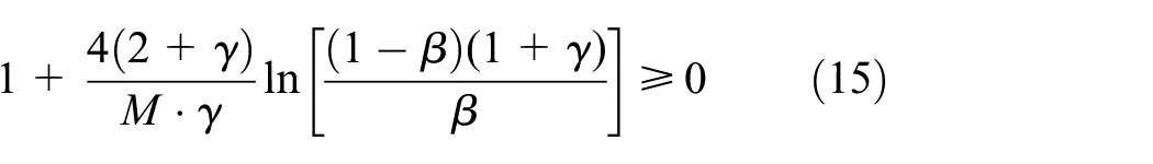
Here, it should be noted that the conditions for the solution of equation (2) should be satisfied according to the following equation

$$1+\frac{4(2+\gamma )}{M·\gamma }\ln \left[\frac{(1-\beta )(1+\gamma )}{\beta }\right]\ge 0$$ (15)

Transform equation (15) type to the following

$$(1+\gamma )·e^{\frac{M·\gamma }{4·(2+\gamma )}}\ge \frac{\beta }{1-\beta }$$ (16)

When the number of sampling points is $M=1024$ and the SNR $\gamma =-20\mathrm{dB}$ , after mathematical derivation, the value of $\beta$ must satisfy $\beta \in (0,0.731)$ , and the equation (16) can be established. The range of $\beta$ values can be extended if the number of sampling points increases. When $M={10}^5$ and $\gamma =-30\mathrm{dB}$ , then $\beta \in (0,0.999)$ . This means that during a sensing cycle and when there is a sufficient number of sampling points (even in the case of low SNR and when the probability of the primary user signal is uncertain), equation (15) is established and there are solutions to equation (14).

Adaptive double energy thresholds

To avoid error judgments due to SNR variations in a received end, lower threshold ${\lambda }_l$ and upper threshold ${\lambda }_h$ are set based on optimal threshold ${\lambda }_o$ (Figure 2). ²⁹ In Figure 2, d is the distance between ${\lambda }_o$ and lower threshold ${\lambda }_l$ or ${\lambda }_o$ and upper threshold ${\lambda }_h$ . The following is thus obtained

$$\{\begin{array}{c}{\lambda }_l={\lambda }_o-d\hfill \\ \multicolumn{1}{c}{{\lambda }_h={\lambda }_o+d}\end{array}$$ (17)

Figure 2.

Double threshold settings.

For weak PU signal detection, threshold ${\lambda }_o$ should be decreased. However, it should not be lower than ${\sigma }_v^2$ . Noise would otherwise be detected as a PU signal. However, ${\lambda }_o$ should not be larger than ${\sigma }_v^2+{\sigma }_s^2$ . The PU signal would otherwise miss detection. To assure a lower probability of false alarm and a higher probability of detection, we thus put a limiting range on threshold ${\lambda }_o$ , as follows

$${\sigma }_v^2\le {\lambda }_o-d$$ (18)

$${\lambda }_o+d\le {\sigma }_v^2+{\sigma }_s^2$$ (19)

Here, equations (18) and (19) gives the following

$$0\le d\le \frac{1}{2}{\sigma }_s^2$$ (20)

Different from conventional double threshold settings, we introduced control parameter $\epsilon$ to accurately fine-tune the double thresholds and define the following

$$d=\epsilon {\sigma }_s^2$$ (21)

According to equation (20), $\epsilon$ satisfies the following

$$0\le \epsilon \le 0.5$$ (22)

When $\epsilon =0$ , it is equivalent to a single threshold case. Thus, ${\lambda }_l$ and ${\lambda }_h$ can be rewritten as follows

$$\{\begin{array}{c}{\lambda }_l={\lambda }_o-\epsilon {\sigma }_s^2\hfill \\ \multicolumn{1}{c}{{\lambda }_h={\lambda }_o+\epsilon {\sigma }_s^2}\end{array}$$ (23)

Parameter $\epsilon$ is an impact factor for double thresholds.

Quantization and coding based on adaptive double energy thresholds

We considered the cognitive radio network as shown in Figure 1. Here, each node communicates with the fusion center. This study assumed that the channel between the node and fusion center was perfect. ${\lambda }_{l,i}$ , ${\lambda }_{l,i}$ , ${\lambda }_{0,i}$ and $w_i$ ( $i=0,1,\dots ,N-1$ ) denote the upper threshold, lower threshold, optimal threshold, and weight of node $E_i$ , respectively.

Calculating bode weights

Assume $E_i$ is the average energy collected by ith node. First, if $E_i$ is not lower than upper threshold ${\lambda }_{h,i}$ and its weight equals 1, then the SU decides that the PU is present. Next, if $E_i$ is not larger than lower threshold ${\lambda }_{l,i}$ and its weight equals 0, then the node decides that the PU is absent. Finally, if $E_i$ is located between ${\lambda }_{h,i}$ and ${\lambda }_{l,i}$ and cannot determine whether the primary user is present, then upper threshold ${\lambda }_{h,i}$ is set as a comparison value. That is, $E_i$ is normalized by ${\lambda }_{h,i}$ and its weight is equal to the normalized result. The weight calculation is expressed as follows

$$\{\begin{array}{c}{w}_i=1,E_i\ge {\lambda }_{h,i}\hfill \\ \multicolumn{1}{c}{w_i=0,E_i\le {\lambda }_{l,i}}\\ \multicolumn{1}{c}{w_i=\frac{E_i}{{\lambda }_{h,i}},{\lambda }_{l,i}<E_i<{\lambda }_{h,i}}\end{array}$$ (24)

where $i=0,1,\dots ,N-1$ is index of SUs, after $N$ nodes performed local spectrum sensing, the $N$ weights form a set $\theta =\{w_0,w_1,\dots ,w_{N-1}\}$ . Figure 3 shows the assigned fusion weights and cooperative spectrum sensing algorithm.

Figure 3.

Assigned weights and the cooperative spectrum sensing algorithm.

According to Figure 3, global sensing performance will change when the two nodal thresholds are altered. According to equation (24), both the weights of the SUs and global sensing performance will change when the two thresholds are altered. As such, it is highly important to select an optimal $\epsilon$ to establish two proper thresholds, thus improving sensing performance. A grid search is conducted to obtain the best parameters for $\epsilon$ in part 4. These are memorized through reinforcement learning strategies to obtain better sensing performance and higher sensing efficiency.

Cooperative spectrum sensing based on quantization and coding

After an SU obtains weight and encodes weight $w_i$ , where $i=0,1,\dots ,N-1$ , the coding rules are as follows: First, if $w_i=1$ , is encoded as 1, and expressed as $C_{i,1}=1,$ then this will be sent to the fusion center, which denotes that an SU transmitted 1 bit of data and consumed 1 unit of energy (e.g. $e_j=1$ ). Next, if $w_i=0,$ is encoded as 0 and expressed as $C_{i,2}=0,$ then this also denotes that an SU sent 1 bit of data to the fusion center and consumed 1 unit of energy. Finally, if $0<w_i<1,$ $C_{i,3}=d_3{d}_2{d}_1$ , where $d_j$ are integers (1 or 0) and $j=1,2,3$ , when $2\times w_i\ge 1$ , $d_3=1$ , otherwise $d_3=0$ , when $2\times (2\times w_i-d_3)\ge 1$ , $d_2=1$ ; otherwise $d_2=0$ , and when $2\times (2\times (2\times w_i-d_3)-d_2)\ge 1$ , $d_1=1$ ; otherwise $d_1=0$ , which denotes that an SU sent 3 bits of data to the fusion center and consumed 3 units of energy.

The fusion center will decode for ${\mathrm{C}}_i$ after receiving sensing results from an SU. Here, the decoding rules can be described as one of three types. First, if ${\mathrm{C}}_i=1$ , then the decoding data are expressed as $D_i=1$ . Second, if $C_i=0$ , then the decoding data are expressed as $D_i=0$ . Third, if $C_i=d_3{d}_2{d}_1$ , then the decoding data are expressed as

$$D_i=\frac{d_3\times 2^2+d_2\times 2^1+d_1\times 2^0}{8}$$

The decoding rules can thus be expressed as follows

$$\{\begin{array}{c}{C}_i=1,D_i=1,\hfill \\ \multicolumn{1}{c}{C_i=0,D_i=0,}\\ \multicolumn{1}{c}{C_i=d_3{d}_2{d}_1,D_i=\frac{d_3\times 2^2+d_2\times 2^1+d_1\times 2^0}{8},}\end{array}$$ (25)

where $0.125\le D_{i,3}\le 0.875$ , and its resolution ratio is 0.125; this can reflect that a node made a contribution for the cooperative spectrum sensing to match its weight.

The fusion center will use majority-rule fusion after completely decoding all data received from all SUs. The fusion expressed is as follows

$$\Re =\sum _i{D}_i,i=0,1,\dots ,\mathrm{N}-1$$ (26)

where ℜ is the fusion result, $i$ is the index of the nodes, and $D_i$ is the decoding data for the node. The fusion center compares ℜ and $N/2$ to decide whether there is a signal from the PU. The expression of this decision is as follows

$$\Re =\sum _{i=0}^{N-1}{D}_i\{\begin{array}{c}\ge \frac{N}{2},H_1\hfill \\ \multicolumn{1}{c}{<\frac{N}{2},H_0}\end{array}$$ (27)

The code algorithm summarizes the coding-based cooperative spectrum sensing.

Coding-based cooperative spectrum sensing algorithm
1: Initialization
calculate $E_i$ , $i=0,1,\dots ,N-1$ , estimate $\left|{\sigma }_v^2\right|$ , set N, M, ${\lambda }_{0,i}$ , calculate ${\lambda }_{l,i}$ and ${\lambda }_{h,i}$ according to (23);
2: Calculate the weights of all SUs
if $E_i\ge {\lambda }_{h,i}$ ; $w_i=1$ ;
else if $E_i\le {\lambda }_{l,i}$ ; $w_i=0$ ;
else $w_i=\frac{E_i}{{\lambda }_{h,i}}$ ;
3: Encode the weights for all SUs
if $w_i=1$ ; $C_i=1$ ;
else if $w_i=0$ ; $C_i=0$ ;
else
if $2\times w_i\ge 1$ ; $d_3=1$ ;
else $d_3=0$ ;
if $2\times (2\times w_i-d_3)\ge 1$ ; $d_2=1$ ;
else $d_2=0$ ;
if $2\times (2\times (2\times w_i-d_3)-d_2)\ge 1$ ; $d_1=1$ ;
else $d_1=0$ ;
$C_i=d_3{d}_2{d}_1$ ;
4: Fusion center decoding for received data from N SUs
if $C_i=1$ ; $D_i=1$ ;
else if $C_i=0$ ; $D_i=0$ ;
else
$D_i=\frac{d_3\times 2^2+d_2\times 2^1+d_1\times 2^0}{8}$ ;
5: Fusion center fuses decoding data on the basis of (26).
6: Fusion center makes decision about PU according to (27).
7: Sensing end

PU: primary user.

For the note code algorithm, the transmission of all SUs combines 1 bit sent and 3 bits sent. As such, the algorithm can improve sensing performance while reducing communication overhead.

Reinforcement learning based on the grid search algorithm

Grid search algorithm

A grid search can be used to obtain optimal $\epsilon$ according to the feedback of global $P_d$ . We conducted a grid search to train parameters in order to improve search efficiency. The trained parameters included SNR (−25 to 0 dB with step 1 dB) and $\epsilon$ (0 to 0.5 with step 0.05). These were saved as a prior knowledge to a knowledge base. Spectrum sensing will then directly invoke optimal $\epsilon$ under an SNR according to the prior knowledge. Figure 4 shows the grid search algorithm used for parameter training.

Figure 4.

Flowchart showing the reinforcement learning scheme based on the grid search algorithm.

In Figure 4, k and j stand for SNR and control parameter $\epsilon$ , respectively; $(k_n,j_n)$ is a prior knowledge group, while $j_n$ is optimal $\epsilon$ under $k_n$ , $n=1,2,\dots ,26$ . If an SNR is newly appearing, then this algorithm will immediately train new parameters; these will be saved as prior knowledge in the knowledge base.

The grid search algorithm process is described as follows

• 1. When an SNR ${\kappa }_i$ appears, the fusion center will conduct a real-time search to find the optimal ${\epsilon }_i$ and obtain the highest $P_d$ . It will then proceed to step 3, where ${\kappa }_i$ is the ith newly appearing SNR and ${\epsilon }_i$ is the corresponding optimal control parameter. These results will be output when $P_d$ and ${\epsilon }_i$ are returned. Furthermore, ${\epsilon }_i$ and ${\kappa }_i$ will become a prior knowledge couple that the fusion center will then learn, for example

$$\phi =f({\epsilon }_i,{\kappa }_{\mathrm{i}})$$ (28)

where $i$ is a positive integer, $\phi$ is a storage library, and $f(·)$ is a learn function.

• 2. When SNR ${\kappa }_i$ is not newly appearing, the fusion center will utilize learned knowledge to directly select optimal ${\epsilon }_i$ ; for example

$${\epsilon }_i=f^{-1}({\kappa }_i,\phi )$$ (29)

where $f^{-1}(·)$ is a function reading knowledge from the storage library.

• 3. Under SNR ${\kappa }_i$ , the range of parameter ${\epsilon }_i$ is divided into 10 equal grids by 11 grid points, ${\epsilon }_{i,j}$ is the jth grid point $j\in \{0,1,2,\dots ,10\}$ . $\mathrm{\Delta }\epsilon =0.05$ is the searching step. The searching process is from ${\epsilon }_{i,0}$ to ${\epsilon }_{i,10}$ with step $\mathrm{\Delta }\epsilon$ .

• 4.  $P_{d,j}$ is $P_d$ of the jth grid point, when a $P_{d,j}=1,j\in \{0,1,2,...,10\}$ , stopping search, the $P_{d,j}$ and corresponding ${\epsilon }_{i,j}$ are returned to 1. The search otherwise continues.

• 5. When the real-time search has been finished, highest probability $P_{d,\max }$ and corresponding optimal parameter ${\epsilon }_{i,j}$ are returned to step 1, as follows

$$\{\begin{array}{c}{P}_{d,max}=max\{P_{d,0},P_{d,1},\dots ,P_{d,10}\}\hfill \\ \multicolumn{1}{c}{{\epsilon }_{i,j}={f_1}^{-1}\left(P_{d,max}\right)}\end{array}$$ (30)

where ${f_1}^{-1}(·)$ is a function seeking ${\epsilon }_{i,j}$ through $P_{d,max}$ .

• 6. End

Reinforcement learning based on the grid search algorithm

The learning process is as follows:

• 1. After the fusion center finishes executing the grid search, the obtained grid coordinates are represented as follows

$$A=\left[\begin{array}{cc}\begin{array}{c}{x}_1\hfill \\ \multicolumn{1}{c}{x_2}\\ \multicolumn{1}{c}{⋮}\\ \multicolumn{1}{c}{x_{40}}\end{array}\hfill & \begin{array}{c}{y}_1\hfill \\ \multicolumn{1}{c}{y_2}\\ \multicolumn{1}{c}{⋮}\\ \multicolumn{1}{c}{y_{40}}\end{array}\hfill \end{array}\right]$$ (31)

The first column in matrix $A$ represents the value of control parameter $\epsilon$ , while the second column represents the value of signal-to-noise ratio $\alpha$ . Each row represents the optimal control parameters found by executing the grid search algorithm in a specific radio environment.

• 2. The fusion center sends matrix $A$ and the matrix description to cognitive users.

• 3. The cognitive user can memorize the data from matrix $A$ ; the local detection threshold is set according to the data and is the best to be preserved. When the radio environment is consistent with the memory, then the optimal threshold in this environment can be directly invoked to perform the next spectrum sensing process.

• 4. In the case of a new radio environment, the fusion center must alter the range of $\alpha$ values and re-execute the grid search algorithm (i.e. execute steps 1-3 again).

Experiments and evaluation

This study designed three groups of Monte Carlo simulation experiments to evaluate the performance of the cooperative spectrum sensing method, as follows: (1) a comparison of detection probabilities ( $P_d$ ) between traditional fusion methods and the new fusion method presented in this article, (2) under the same conditions, a comparison of probability of error ( $P_e$ ) between the used grid search algorithm and those unused in this article, (3) under the same conditions, a comparison of sensing speed between reinforcement learning and non-reinforcement learning, (4) verification of fast fusion algorithm, compare the processing time of using fast fusion algorithm with that of not using fast fusion algorithm. The Monte Carlo simulations were conducted under conditions involving path loss and additive Gaussian white noise.

The simulation experiments set the PU signal to a BPSK, bandwidth to 100 kHz, and sensing duration to 100 ms. ³⁰ The PU was placed in the center of a 1000 × 1,000 m square and surrounded by 16 evenly distributed sensing nodes. The simulation scenario is shown in Figure 1. The probability of setting the channel of PU occupancy was $\beta =50\mathrm{\%}$ , while the transmitting power of the PU signal was 100 mW. ³¹ Each node sampled 20 points; the noise power range was set to between 0 and 2 dB, while the path-loss exponent was 2.7, the standard deviation of the shadow was 5 dB, and the mean of the multipath Rayleigh fading was 1.^32–34

Figure 5 illustrates a comparison of detection probabilities ( $P_d$ ) between the traditional fusion methods and the new fusion method proposed in this article. The traditional methods used for comparison included AND, OR and Majority fusion methods. As seen in Figure 5, the detection probability ( $P_d$ ) obtained by the new fusion method was higher than that obtained by traditional methods. This is more obvious in cases involving low SNR because each sensing node uses double the threshold energy detection and calculates weights according to the signal energy received by itself. Such nodes can then make appropriate contributions to the spectrum sensing process based on their own weights. As such, the new fusion method more accurately reflects the actual roles of each node when compared to traditional methods.

Figure 5.

Comparison the traditional fusion methods and the new fusion method.

Figure 6 illustrates the comparison of probability of error ( $P_e$ ) between the grid search algorithm used in this study and other algorithms (i.e. fixed-single and fixed-double threshold algorithms). As seen in Figure 6, the grid search algorithm exhibited the lowest error probability during spectrum sensing. This is because the best detection threshold can be obtained through the grid search algorithm in any radio environment. The other two algorithms have fixed thresholds and can therefore not adapt to noise fluctuations. While the probability of error ( $P_e$ ) increases when SNR decreases in all cases, the grid search algorithm results in the smallest increase.

Figure 6.

A comparison of probability of error between the grid search algorithm and others.

Figure 7 shows a sensing speed comparison between reinforcement and non-reinforcement learning. As seen, reinforcement learning takes less sensing time than non-reinforcement learning under the same SNR conditions. This is because reinforcement learning can directly invoke detection thresholds in the same environment from the repository. If reinforcement learning is not used, then every spectrum sensing procedure requires a grid search algorithm to find the optimal threshold; this requires more sensing time. Sensing time decreases when SNR increases because the radio environment is simpler; with an increased signal-to-noise ratio, less information is stored and judgments are easier to make.

Figure 7.

A sensing speed comparison between reinforcement and non-reinforcement learning.

In order to verification of fast fusion algorithm, compare the processing time of using fast fusion algorithm with that of not using fast fusion algorithm. The experiments are all under the same number of nodes. In order to highlight the advantages of the fast algorithm proposed in this article, observe the data processing time under different node numbers. Table 1 shows the processing time at different nodes. The processing environment is MATLAB 7.0, and the computer configuration is Intel (R) Core (TM) i5-8500 CPU at 3.00 GHz, RAM is 8 GB, and 64-bit operation system.

Table 1.

compare the processing time of using fast fusion algorithm with that of not using fast fusion algorithm.

Number of nodes	Processing time using fast fusion algorithm (ms)	Processing time do not using fast fusion algorithm (ms)
5	0.32	0.38
10	0.56	0.64
15	0.72	0.79
20	0.84	0.92
25	0.95	1.04
30	1.02	1.16

It can be seen from Table 1 that the fast algorithm used by the fusion center can effectively reduce the data processing time, and the average processing time can be reduced by 18%. When the number of nodes is more, the advantage of fast algorithm in dealing with big data is more obvious. When the number of nodes is more than 30, the time of fast algorithm in dealing with data is less than that of not using fast algorithm in dealing with 25 nodes, which can be the advantage of fast algorithm in this article.

Conclusion

This article studies a new perceptual data fusion algorithm, which can process the perceptual data of each node quickly without delay. In the cognitive radio network, different nodes have different perception data due to different geographical location, and the contribution of each node’s perception data to cooperative perception is also different. The fusion center uses reinforcement learning mechanism to select cooperation nodes by identifying the sensing performance of node, which can reduce the processing data to a certain extent, and enable the fusion center to process quickly the data sent by each node will not cause decision delay. This greatly improves the throughput of cognitive users while protecting the primary users. The experimental results show that the big data fast fusion algorithm in this article can effectively reduce the data processing time, The average processing time of using fast algorithm is 18% less than that of not using fast algorithm. When the number of nodes is more than 30, the time of fast algorithm in dealing with data is less than that of not using fast algorithm in dealing with 25 nodes, which can be the advantage of fast algorithm in this article. Furthermore, the algorithm in this article can reduce the processing time of node data and improve the sensing performance at the same time and increase the throughput of cognitive users, which is of great significance. However, at present, only the fast algorithm of big data is implemented in the fusion center, but not the energy-saving algorithm in the node itself, which is the follow-up research goal.