Sage Journals: Discover world-class research

Abstract

Low-power lossy networks performance relies heavily on the wireless node battery status. Furthermore, Routing Protocol for Low-Power and Lossy Network routing protocol was not optimally designed with sustainable energy consumption in mind to suit these networks. Prolonging the lifespan of these networks is of utmost priority. This article introduces a solar energy harvesting module to power energy-constrained network devices and quantifies the effect of using harvested energy on prolonging their network lifetime when Routing Protocol for Low-Power and Lossy Network routing protocol is used. Simulation of the new developed module is conducted in three different scenarios using Contiki Cooja simulator sporting Zolertia Z1 motes. Furthermore, the harvested energy used was fed from a Cooja-based Simulation model of actual PV supercapacitor circuit design. All battery levels were set to 1% of their total capacity for all nodes in the network to speed up observing the energy harvesting effect. The performance evaluation results showed that the network with no-energy harvesting operated for time duration of 4:08:04 time units (i.e. hour:minute:second) with a dramatic decrease in connection between nodes in the network. However, the same network, when using the harvested energy to back up the battery operation, lasted for 6:40:01 in time units with improved connectivity, a total extended network lifetime of 2:31:97-time units. Furthermore, for the Routing Protocol for Low-Power and Lossy Network routing metrics, OF0 outperformed ETX in term of throughput, packet delivery ratio, energy consumption, and network connectivity. Results indicate that the developed harvested energy module fits perfectly for any Cooja-based simulation and mimics actual photovoltaic-based supercapacitor battery. It should also help researchers introduce and quantify accurately new energy consumption-based routing metrics for Routing Protocol for Low-Power and Lossy Network.

Keywords

IoT WSN low-power lossy network Routing Protocol for Low-Power and Lossy Network energy harvesting network lifespan

Introduction

Internet of Things (IoT)¹ is one of the most important technologies of the future that are expected to make a big change in the world around us by allowing communication between objects “things” to do daily activities instead of humans. Wireless sensor networks (WSNs), an enabling technology for IoT, consist of many heterogeneous devices (sensors) which communicate autonomously.²

Basically, WSN is a network made by a large number of sensor nodes where each sensor is linked to a node. The sensor node has several parts responsible for receiving, processing and sending data to a server or even a cloud computing service host. These nodes usually have small scale radio transceiver possessing its own antenna to secure the process of sending data, a microcontroller for data acquisition and processing. It also has a built-in analogue/digital electronic circuit known as signal conditioner circuit meant to translate the nature of sensed data signal to a form that suits the microcontroller acquisition ability. Apart from that, the node has its own power source, usually batteries, supercapacitors or any sort of power harvesting system.³ The reading acquired by sensor nodes is gathered by a gateway to be passed to a server or host.⁴ In addition, routing the data in such environment was a challenge because of constrained sources of the power source. Therefore, Routing Protocol for Low-Power and Lossy Network (RPL) was formed by Internet Engineering Task Force (IETF) to develop an adapted routing solution for such networks that contain large number of constrained nodes with limited processing, power, memory. This kind of network is called low power lossy network (LLNs) and the LLNs terminology is used to indicate the focus of routing over low-power and lossy (ROLL) group. RPL is IPv6 routing protocol for low-power and Lossy network that focuses on path selection while considering the routing behavior. The objective function is the metric that is used to determine the perfect way to route the packets of data from node to other node toward the sink node, the node with small rank called child while the node with high rank called parent. Each node wants to send data can communicate with ambient nodes and choose the one that at close distance to it and links it to other nodes to the sink node. Furthermore, LLNs are naturally constrained network, which consequently include low throughput, high packet loss, high latency, and lack of IP service.

Routing protocols in WSN are classified into two types: Reactive and Proactive. Reactive protocols transmit data if there is a need of route by path of data in such network, otherwise, they do not work. However, this would consume more energy due to long time spent for finding routes when needed by data. Such example of these protocols, ADOV,⁵ DSR,⁶ and TORA.⁷

In contrast, Proactive protocols are ready to provide routes of paths of data before they require it. This kind of protocols is represented in RPL routing Protocol. Thus, RPL is routing protocols that makes use of IPV6 a standard for WSN. It has been designed by ITEF as routing protocol that rout over Low Power Lossy network (ROLL). So, one of the key issues and important part is selecting the objective function which is used to find the suitable path to the sink node. Likewise, Objective function is defined as a metric which helps node to find and select a parent from node’s neighbors. RPL has two main objective functions namely Minimum Rank with Hysteresis Objective Function (MRHOF) and objective function zero (OF0).^8,9

The power source of constrained energy devices operating in these LLNs is typically batteries which deplete its energy over short time. Furthermore, changing these batteries periodically is very difficult process especially in remote area where a huge number of sensor nodes are deployed. Therefore, energy harvesting for WSN¹⁰ is considered a good solution to convert ambient energy into electric energy that can be used to power low power devices to prolong battery age. Energy harvesting or energy scavenging is a term used to describe the process of capturing ambient energy such as, wind, thermal, vibration, RF signals, and solar energy, and store this small, captured amount of energy into power bank and use it to power sensor nodes in WSN. Energy storage devices in WSN are often rechargeable batteries as well as supercapacitors.

In this article, we investigate the effect of adding energy harvesting module (EH-Module) on prolonging network lifespan when RPL routing protocol is in use. EH-module is developed to simulate RPL network in Contiki Cooja simulator.¹¹ This module is an extension of PowertraceK that is used to provide neutral operation of the minimum energy node in Energy-Harvesting Environments.¹² However, our developed module combines three sub-modules into one module. These sub-modules are consumption sub-module, storage sub-module, and harvesting sub-module. We developed this EH-module to harvest real data of solar energy accumulated by Colombia University.¹³ Furthermore, this study provides a comprehensive evaluation for RPL standard objective functions in term of energy harvesting. This is to our best knowledge is the first RPL evaluation with and without energy harvesting for both OF0 and ETX. To evaluate RPL metrics performance in term of prolonging network lifetime, three network populations of 100 nodes, 50 nodes, and 25 nodes are designed. Each network population will cover both objective functions; ETX and OF0 with and without energy harvesting as power source.

Contiki¹⁴ contains many examples that are ready to be run in Cooja simulator. These examples are very helpful for those who are new to Contiki, so as it is easy for them to modify it regarding to their project requirements. For example, UDP RPL is an example used to form a network of many motes that use RPL routing protocol with UDP protocol for network layer. Simply, programs or applications in Contiki are written in syntax of C language in *.c files. These files then compiled to obtain a binary file. It converts the syntax in C language into binary to be used in a certain hardware target or it could be run in Contiki simulator to validate the effectiveness of such program.

The paper structured as follow. Related work and simulation module implementation are highlighted in sections “Related work” and “Energy-traced harvesting simulation module implementation,” respectively. Sections “Network simulation and modelling” and “Performance evaluation” present the performance evaluation and results. Section “Conclusion” elaborates the conclusion.

Related work

Several works have been conducted proposing the use energy harvesting modules in the aim to prolong the life spam of autonomous sensing nodes in WSNs. These works differ in the type of renewable energy source used for the harvesting module as well as its architecture. However, to our knowledge, all of the so far proposed modules were using purely experimental or mathematically deduced power trace. In this work, we have designed and developed a simulation model based on actual experimental circuit setup for a PV energy harvesting module. The simulation module was integrated into Cooja simulator such that it can be attached to the sensor node to facilitate mimicking actual WSN scenarios. The details of the circuit setup and the simulation model for the energy harvesting module is presented in detail in section 3 below.

The main contribution of this paper is three folds. The introduction of a real-life simulation model of energy harvesting module based on PV supercapacitor battery circuit to the popular Cooja simulation environment. The integration of the developed module with any sensor node within Cooja simulation environment. The evaluation of the newly introduce simulation module’s contribution to the network as well as sensor node battery lifespans.

Due to the inexistence of such module modeled in Cooja simulator, the challenge raised by extending Cooja source code accordingly, and the functioning of Contiki operating system, this energy harvesting module was developed. The main advantage of the proposed module is that it gives a blueprint to future research to use Cooja simulator for modeling energy harvesting–enabled WSNs. However, the main disadvantage it only considers PV-based supercapacitor circuit configuration (Table 1).

Table 1.

Comparison of energy harvesting modules in related works.

Work	Harvested Energy Trace type
Hou et al.¹⁵	Experimental trace data
Zhang et al.¹⁶	Experimental trace data
Deng et al.¹⁷	Experimental trace data
Chamanian et al.¹⁸	Mathematical model generated data
Hadas et al.¹⁹	Mathematical model generated data
Our proposed approach	Cooja-based Simulation model of actual PV supercapacitor circuit design

Even though the works most related to ours are those proposing solar energy harvesting module to prolong WSNs lifetime. However, beyond that many other works have been published about the integration of EH in WSNs, each set covering some aspects on the wide subject. In Varga et al.,²⁰ the author proposed a stack of network protocols specially meant for energy harvesting enabled WSNs, the author presented results was the power consumption using his proposed stack of protocols compared to the network power consumption when using standard protocols. Similarly, Chiti et al.,²¹ Sarwar et al.,²² and Liu et al.²³ focused on proposing greener RPL protocol, for which nodes power consumption is more efficient and thus can be suitable for autonomous and EH enabled WSNs. Other works which may be considered relevant to ours are the studies by Liu et al., Lu et al., and Clerckx et al.,^24–26 which all proposed RF energy harvesting methods, this may be relevant since WSNs’ nodes do have an RF module which is the module having the highest power consumption.

Energy-traced harvesting simulation module implementation

For simulating a wireless LLN design with RPL routing protocol and energy harvesting, we have developed an energy harvesting model as a part of existed energy estimation tool “PowertraceK.” Hence, in this section, we provide an extensive details of energy harvesting module in terms of design and implementation.

Design and implementation

In this section, we elaborate the development procedure and steps for the energy harvesting module (Figure 1). Our developed module is an extension for PowertraceK presented in Riker et al.¹²

Figure 1.

Energy harvesting module architecture.

Do{-State1 (supercapacitor charging/ single power source: non chargeable):-State2 (hybrid mode: switching between the two power sources) If (non chargeable battery ! = empty & chargeable battery == empty) { Goto State 1 }Elseif ((non chargeable battery == empty & chargeable battery == empty){Node == deadBreak;} else{-state3 (single power source: supercapacitor)}While(true)

The model encompasses an energy storage element, which is a supercapacitor charged using a renewable energy module, in our case it is a PV solar panel. The sensor node would be having a hybrid power source for powering its RF module used for packet transmission and reception. The RF module would be powered by switching between the non-chargeable power source and the supercapacitor battery. The life cycle of the sensor node would be as follows:

Switching between the states would be enabled according to the following circuit:

Do{Pin 4: input // controlling capacitor output voltage.Pin 3: output //controlling the switch linking the capacitor to the charging modulePin 5: output // selecting the power sourceBool capacitor-charging: true;Pin 4 = 1;if (pin 4 == Vcmax)// capacitor fully charged{ capacitor-charging: false;// set capacitor to discharging mode pin 3 = 0; // delink the connection between capacitor and charging module}If (! capacitor-charging && pin 4 == Vcmin) // capacitor discharged{ capacitor-charging: true;// set capacitor to charging //mode pin 3 = 0; // link the connection between capacitor and charging module}If(capacitor-charging){Pin 5 = 0;// single power source (non chargeable battery)}If(!capacitor-charging){Pin 5 = generate-PWM(T, DC);// generate a pulse width modulation signal with //period T and Duty cycle DC, to switch between the two batteries in a periodic //manner}//While(true).

As illustrated in Figure 2, Pin 3 of the microcontroller is set as an input, sensing the super capacitor voltage, pin 4 is set as an output controlling a MOSFET transistor switch, linking the capacitor with the charging module. Pin 5 is set as an output controlling the selection pin of the multiplexer, which decides which source would be powering the node Rf module.

Figure 2.

Hybrid energy source for the sensor node.

The microcontroller logic is according to the following pseudocode:

To model the circuit described in Figure 2, as well as its logic described above in cooja simulator, we used two existing modules in the simulator which are the PowerTrace module as well as the C-Timer call back timer module.

The power trace module tracks the sensor nodes battery power consumption. There are three types of power consumption modeled in Cooja. They are the packet transmission power consumption deducted each time the node sends a packet, the packet reception power consumption deducted each time the node receives a packet, as well as the idle power consumption. To module the supercapacitor battery energy consumption we created a second power trace module identical to the original one. The appropriate power trace module is called upon time triggered events using Cooja call back timer module, according to the previously described logic.

The call back timer module takes two parameters:

An expiration time: after this defined time elapses after calling the timer, it triggers the call back function to be run.

Call back function: this parameter is a reference to a call back function that is supposed to be executed after the timer expiry.

This module has been used to set the state of the supercapacitor to charging or discharging. The charging as well as discharging time of the supercapacitor battery is computed according to the following expressions

$T_{charging} = 38 \times R \times C$ (1)

$T_{discharging} = 40 \times R \times C$ (2)

Therefore, the Ctimer function would be taking these parameters as follows:

If (capacitor-charging){ Ctimer(T_charging, Call_back_function) } Else{ Ctimer(T_discharging, Call_back_function) } Where the call back function just toggles the state of the capacitor. Call_back_Function(){ Toggle(capacitor-charging) }

In the file where Power Trace module is called, the appropriate Power Trace module is called according to the following logic:

If (capacitor-charging){ Powertrace() // the original power trace module is called //corresponding to the non chargeable power source }Else// switching between the two batteries in a periodic manner{Ctimer(T, Call_back_fuction)Powertrace()}Call_back_function(){Powertrace1()// calling the created power trace correspondingto the //rechargeable batterie}

Network simulation and modelling

It is necessary to evaluate our developed module with different RPL network populations. We choose RPL routing protocol to be evaluated when energy harvesting module is added to the battery. This is done to investigate the effect of energy harvesting on prolonging RPL LLN lifespan as it is the preferred routing protocol in LLNs part of the IoT. In addition, to the best of our knowledge, RPL metrics were not evaluated in energy harvesting LLNs settings.

Simulation model and network setup

To test and evaluate the developed energy harvesting module, different networks populations, that use RPL routing protocol, are designed, and implemented in the Cooja simulator. The motes are set of clients and one server, in each network node population. Each client node acts as a child or parent node in DODAG setting (see Figure 3(a)), while server mote represents root node for the same DODAG. In these experiments, we use Contiki udp-rpl case study. This case implements UDP over RPL and it uses a UDP server as the root node that receives packets from the sender nodes. Client nodes are UDP clients representing sender nodes that periodically send packets to server via single hope or multi-hop. Furthermore, the Contiki radio channel UDGM is used. This radio model provides path loss calculation due to transmission distance and success ratio.

Figure 3.

(a) DODAG setting example and (b) network of 100 motes in Contiki Cooja.

Consequently, to investigate the network from various aspects, different objective functions of RPL protocol are used. First, the network was set with ETX (Expected Transmission Count), and then, it was changed to OF0 objective function. In the simulated network, nodes were connected to each other and they send packets to the sink node in the network periodically. The packet is sent from the client nodes to the server node every 30 s with a payload of 240 bps.

Three network populations of 100, 50, and 20 motes are distributed equally on the network grid. Figure 3(b) represents a network of 100 nodes in Contiki Cooja simulator. Each network population is implemented with four experiment simulations with different battery methods as well as varied RPL objective functions. All networks use only grid topology within 200 square meters. Table 2 shows the parameters which are typically determined for each simulation test.

Table 2.

Simulation parameters.

Parameters	Value
Propagation model	UDGM
Mote type	Zolertia Z1 mote
Network Layer	IPV6 + 6loWPAN
Transport protocol	UDP
Mac layer	ContikiMAC
Sending Interval	30 s
Node population	100, 50, 20
RX, & TX range	100 m
Node distribution	Grid
Mote startup delays	1.000 ms
Objective function	OF0 & ETX
Wireless	IEEE 802.15.4
Packet size	30 bytes

OF: objective function; ETX: expected transmission count.

Battery powered method

Low power devices or constrained sensor nodes are usually powered with batteries due to different reasons. These batteries must be suitable for small size of the embedded devices and must operate for the longest time possible. Therefore, in our study, we focused on using energy harvesting for charging theses batteries. For comparison purposes, we examined the various network node populations, either with battery only (non-energy harvesting) or battery with energy harvesting.

No-energy harvesting mode

In no-energy harvesting mode, each node in the network is powered solely by its own battery. To implement this in Cooja simulator, Powertrace system²⁷ is used to estimate power consumption in low-power devices. The extension version of Powertrace, PowertraceK system, is used to estimate energy consumption as well as residual energy in each battery node. PowertraceK added the Kinetic battery model to the original Powertrace tool. Kinetic battery model (KiBaM) estimates the battery lifetime by calculating many related parameters for the state of the charge (SoC) in the battery. It considers that the battery stores the charges in two different methods, either immediately available charge, or bound chemically charge. The battery capacity can is altered by setting a maximum amount of charge as required. In this study, a battery capacity of 800 mAh is used for Zolertia motes. Thus, the residual energy represents the battery capacity that decreases periodically due to mote energy consumption.

Energy harvesting mode

This mode represents the harvesting sub-module combined with the KiBaM model to increase battery residual energy periodically. In this method, we assumed that battery model has a constant value of charge that acts as battery capacity. This battery capacity is consumed frequently by operating mote components such as CPU and transceiver. However, energy harvesting module use a real data values from the trace file of indoor PV harvested energy. Once these values are added to the available charge in KiBaM model, the residual energy is increased. Energy harvesting module typically required to set up a time for harvester value to be added to the battery. In this study, time was set up to include the harvested values to the battery after every 1-min duration. According to data trace file, the harvested values were accumulated every 30 s. Therefore, set up time should not be less than harvester time to a reliable system.

Measuring performance metrics

To measure performance parameters for RPL metrics, this section illustrates in a step-by-step approach how to calculate each parameter. Three RPL network populations were designed in Cooja simulator and tested extensively to fulfill the evaluation and benchmarking for RPL with and without energy harvesting capability. Therefore, each network in Cooja simulator operates in full connectivity, where client node sends a packet to the root node every 30 s, which is the send interval for all the nodes in the network. Cooja terminal output is used to illustrate network behavior for each node with varied ID. Each node ID presents the timestamp for sending a packet while root node notifies that it has successfully received the packet.

Basically, network lifespan is the time of network simulation from the start of simulation until the whole network is dead. It has been calculated as a function of the simulation time, where it is divided into three rounds. The first round is from start of simulation until the time for the first node to die (FND), second round is from FND time until the time when half of the population dies (HND), and the last round is from HND until the time for last node to die (LND). According to our developed module, it uses energy consumption sub-module to read battery residual energy periodically. Residual energy is updated every minute for every individual mote. A node is considered dead when residual energy is equal to or less than 10 uWh.

Throughput is defined as the rate of successfully transmitted data for a specific time (in bps—bits per sec or pps—packets per second) from one node to the other one within the network for specific duration of simulation time. Thus, equation (1) is used to calculate throughput parameter for all nodes in the RPL network

$Throughput = SRP \times packet size / T_{s}$ (3)

where SRP is successfully packets received and T_s is the simulation time. In this case, we sum the successful received packets at root node for every period as you wish which consider the simulation time. The packet size of 30 bytes is the default value in our UDP client model for all sender nodes and throughput is computed in bit per second as well as in packets per second.

Packet delivery ratio (PDR) is simply defined as the ratio of SPR to the total number of sent packets, and it is computed by dividing the number of SPR at root node by total packets sent by sender nodes. In this case, each node sends a packet periodically based on the set up send interval. Therefore, PDR is computed as follows

$PDR = SPR / Total Sent packets \times 100$ (4)

Energy consumption is the amount of energy used by the components of sensor mote such CPU, transceiver, and sensor actuator. And it typically calculated by the developed EH module. Therefore, the concept of calculating energy consumption is simply determining the current drawn by the specific mote type used in the simulation. Zolertia datasheet was used to determine the amount of current drawn by each mode such as idle mode, low power mode, and sleep mode. Voltage is also stated at the battery used to power the node. In our case, voltage is 3.7 V for Zolertia mote. Furthermore, energy consumption is computed during a specific period. The following equation is used to compute energy consumption

$Energy Consumption = I \times V \times time$ (5)

where I is current draw at different mode in the mote components, V represents voltage available for the used battery mote, and time is the duration when the node is ON. Furthermore, residual energy is also computed depending on energy consumption, the amount of energy consumed in every state is subtracted from battery residual energy.

Performance evaluation

Lossy low power network lifespan

Network lifespan can be determined through parameters like network coverage and connectivity or when the node battery is drained. Therefore, in our case, we obtained the network lifespan depending on the residual energy for each node battery in the network. The battery is considered with full capacity at the beginning of the simulation session and is reduced after each activity. Often, each node behaves differently, and this relies on its location in the network. This also leads to diverse behavior of batteries for each node. Due to the lengthy process of simulation to drain a node battery with 800 mAh, all node batteries were set to 1% of their maximum capacity only, rather than the maximum battery capacity. This will speed up draining the batteries and reduce the consumed time, memory resources, and computational load needed to run the simulation.

In the simulation test of the network with 100 nodes, Figure 4 shows network lifespan when the RPL protocol operating with ETX objective function. In network with no-energy harvesting, the first node drained its battery at the time of 34:02 (34 min and 2 s). While in network with energy harvesting, first node has been exhausted at the time 36:01 (36 min and 1 s). It is clearly seen that network with energy harvesting has slight increase in network lifespan due to battery extension caused by energy harvesting. Furthermore, several nodes rely on its central parent to send their data to the sink node. However, theses nodes become out of coverage once the battery of central parent node is exhausted. Therefore, around 87 nodes in the network lost their connection within the first hour due to battery depletion and other nodes become out of coverage. First round (FND) shows slight difference in network lifespan because both networks operate with very low battery capacity of 1% only.

Figure 4.

Network lifespan for objective function (ETX).

Second round is represented by (HND) where half of the nodes of the network has died. Network with energy harvesting also appears with longer lifetime compared to no-energy harvesting where the power source is only battery. At time of 0:52:01, half of the nodes have exhausted their battery energy for nodes with energy harvesting, while in the network that operates with no-energy harvesting, the second round occurred at time of 0:44:01. Then, the network has continuously adjusted its connectivity graph and stabilized for a period between first hour and second hour. The connected nodes at this period were around 18 nodes only before a sudden loss happened successively that made the number of live nodes drop to a mere three in the network. This has continued until the death of last node (LND) at the time of 4:08:01 with no-energy harvesting and at time of 6:40:01 with energy harvesting. A promising advantage of more than two and a half hours is evident for the energy harvesting with the battery for a mere simulation time of 1% of the maximum battery capacity. This is obviously expected to translate to roughly several days of continued operation if energy harvesting continued for the 100% of the maximum battery capacity at the nodes.

Furthermore, when ETX routing objective function is used, the extended network lifetime is 2:31:97 (2 h and 31 min and 97 s) at LND. However, for this last period of network survival, the least number of nodes operate in this round (HND ≥ LND) in network, and therefore, energy consumption due to communication and routing is also less, even though the amount of harvested energy in the network is also small.

However, when the routing objective function is changed to (OF0) for the RPL protocol, a different set of results is obtained. Figure 5 shows the performance of an LLN with two methods of energy supply, battery only and battery with energy harvesting. Initially, the network powered by battery without energy harvesting, operates with a full connectivity between all nodes until the FND depleted its battery energy at the time of 36:01 (36 min and 1 s). Like ETX results in Figure 4, the FND is the node that once connected many nodes to the sink. Once died, many nodes struggled to connect to the sink due to the grid topology used as they became further away from the sink and out of the communication range. Several nodes failed to find an alternative route and hence became disconnected from the network. The simulator then considers their battery supply depleted and removes them from the simulation. Then, the network functionality was on with a small number of active nodes until the last node was dead at the time of 8:08:01. In contrast, when the energy harvesting module is attached to the battery model, the network lifespan has been extended approximately to 3 extra hours. That was clearly seen in the graph in Figure 5, whereas the first battery node is drained at 50:01 (50 min and 1 s), while the last node is being exhausted at 11:19:01 (11 h and 19 min and 1 s).

Figure 5.

Network lifespan for objective function zero (OF0).

Generally, most of the battery nodes become drained and/or lost their network connection at the first and second hour for both objective functions with and without energy harvesting.

In Figures 6 and 7, it is clearly seen that the network with energy harvesting shows a better performance in terms of lifespan for both objective functions; ETX and OF0 than using only battery as a power source. Furthermore, objective function zero (OF0) illustrated longer lifespan compared to minimum rank with hysteresis objective function (ETX) for all different network node populations. This mainly because the ETX consumes more energy due to the many operations needed to determine the preferred parent for each node. Moreover, the battery depletion of central parent node might cause a sudden cutoff in the network, and thus, children nodes lose their connections with root node. So, the child node needs to go through extra computation and communication operations to find another preferred parent. These operations need to turn on duty cycle for longer time, and thus more power consumption is needed. This is especially true for ETX that is always looking for the optimal path to reach the root node. In addition, number of duplicate and lost packets is high in ETX leading to more energy consumption and consequently shortage in the network lifespan. Furthermore, the ETX Objective Function demands an intensive computation to define the minimum overall ETX to the root node. This is due to high packet loss and more frequent retransmissions, which require longer time and consume power resource. However, OF0 routing in RPL enabled network outperforms ETX in terms of network lifetime in different network node populations because it needs fewer operations to calculate the hop counts to the root node to determine the optimal path. This is translated to less time for the duty cycle and hence longer extension of the battery life.

Figure 6.

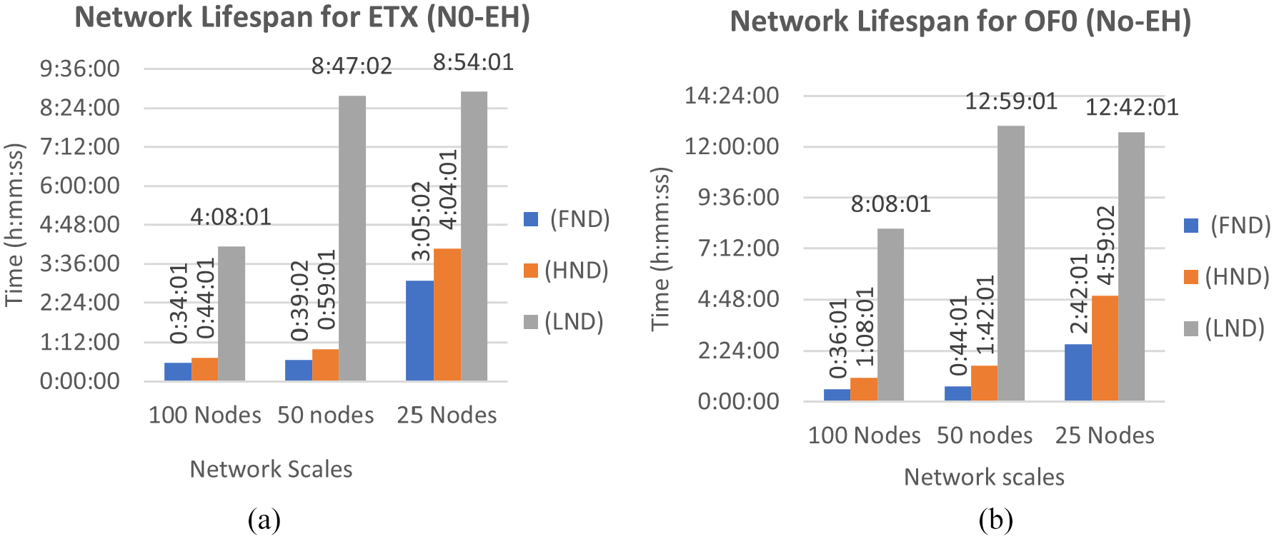
Network lifespan for both (a) ETX and (b) OF0 without energy harvesting.

Figure 7.

Network lifespan for both (a) ETX and (b) OF0 with energy harvesting.

Throughput

Throughput is calculated in bits per second at a rate of 1 reading every 5 min. Both ETX and OF0 were evaluated. Evaluating these objective functions in terms of throughput while using energy harvesting module is going to optimize RPL routing protocol objective functions. The first 5 min of simulation time were dropped from the calculation of the throughput to increase the accuracy of the results. Figure 8 shows throughput performance for the ETX enabled network of 100 nodes. The ETX Objective Function will attempt to find an optimal path to send and receive the data over it. Figure 8 illustrates the throughput for the OF0 enabled network for both power modes of with and without energy harvesting. Accordingly, energy harvesting network illustrates improvement in the throughput rate for both ETX and OF0. It is seen for both ETX and OF0 that network throughput started at a very high rate, and then it shows some fluctuation due to interference from neighboring nodes which send and receive packets periodically. Furthermore, the network was fully connected at the beginning and then nodes started to lose their connection with the network due to battery energy depletion until the network operates only with two nodes. This clarifies that network throughput is affected by network connection. The more nodes connected the more packets are received and thus high throughput rate and vice versa. As shown in Figures 8 and 9, network throughput for OF0 outperformed the network throughput for ETX objective function. At the beginning, OF0 provides throughput rate of 512 bps with no energy harvesting and 587 bps with energy harvesting. However, ETX Objective Function shows throughput of 190 bps with battery only and 297 bps with energy harvesting module. The throughput is then decreased eventually until it reached 8 bps with two nodes connected only.

Figure 8.

Throughput for objective function (ETX).

Figure 9.

Throughput for objective function (OF0).

To provide a comprehensive evaluation for standard objective functions in RPL protocol, we analyzed the network throughput in three different network node populations for both ETX and OF0, as shown in Figure 10. Generally, OF0 shows better performance of throughput than ETX Objective Function in 100 nodes network population. This is obviously related to high performance for OF0 in dense network and unreliability for OF0, which does not require long time to send data. ETX, however, is more reliable and needs a time to send a reliable data through more retransmission. This might cause a network congestion and high packet drop. However, ETX objective function with energy harvesting shows higher throughput than without energy harvesting. This is mainly because energy harvesting provides longer time, which asserts ETX to send more packets in reliable manner. OF0, however, shows similar behavior in term of throughput between both battery methods, with and without energy harvesting.

Figure 10.

Total network throughput for each round with three different node populations.

In network population of 50 nodes, throughput rate is also showing that OF0 is better than ETX Objective Function with and without energy harvesting for first and second rounds, while the last round shows similar throughput performance. This is obviously due to the last two nodes connected to the network. Since ETX operates in low density network with less radio overlapping, energy harvesting mode extends the network lifetime. Surprisingly, no energy harvesting mode outperforms energy harvesting mode because less time with very high packet received can produce a high throughput. On the other side, network with 25 nodes demonstrates similar throughput performance for both ETX and OF0 with and without energy harvesting. This is probably due to the shortage of battery capacity that we have used for each node in the network. Interestingly, smaller network density produces an optimal performance for most of the network metrics. Therefore, network status would be changed over the time, and thus, metrics are frequently altered similarly.

Packet delivery ratio

Packet delivery ratio is found to be very low when the network is dense network with 100 nodes deployed in 200 square meters area due to physical network topology instability.²⁸ Figure 11 shows how the packet delivery ratio is increased dramatically at third round in ETX routing, as network becomes of lower density. At the third round, network contains lesser nodes connected to the sink, and so, it is more reliable for sender nodes to send packets to the root node with no delay, lesser forwarding and hence no packet drops, since there is lesser radio interference from neighboring nodes and no traffic congestion for data. Energy harvesting method shows a slight improvement respecting packet delivery ration due the extension in the network lifespan. From Figure 11, OF0 performs better than ETX in terms of packet delivery ratio in dense network, as with ETX nodes experience frequent congestion and collisions. Furthermore, packet drop might be caused by many other reasons such as network density, short send interval, radio interfaces, ETX reliability, and too many destinations with same minimum rank. Hence, dense networks with bad link quality may be more suitable for OF0 routing rather than ETX.²⁹

Figure 11.

Packet delivery ratio.

Consequently, as network size decreases, the packet delivery ratio increases. This is true for networks with 50 nodes and 25 nodes populations. However, at lesser dense network, both ETX and OF0 have similar performance with slight advantage to ETX due to its reliability in low density network, that works to send packets periodically with very few packet drops. When comparing the performance of PDR with and without energy harvesting, 100 nodes network has a clear difference for the same objective function. Energy harvesting prolongs the lifespan of the network and that affects the PDR performance slightly positively for all network population sizes. However, as the send interval is set to 30 s, each node may send packets to the root node every 30 s and this is considered very constrained for LLNs.

In general, with energy harvesting, OF0 demonstrates similar performance of packet delivery ratio to ETX objective function for low density network (e.g. during the FND round) as it might reach close to 100% for the LND round.

Energy consumption

Energy consumption is very critical issue in LLNs, as this is referred to as a constrained power source in WSNs. Therefore, power consumption analysis is useful to optimize RPL routing protocol in LLNs. In this study, we calculate a periodic energy consumption for every minute. This was done with the help of Energest module in Contiki operation system.

Figure 12 shows the energy consumption for the first node to die due to its battery depletion. The figure shows the energy consumption for both ETX and OF0 objective functions. When the network has a high density of nodes, the power consumption is as high as 60.4 uWh. However, it reduces drastically as the network population becomes lighter. What is interesting is that energy harvesting has almost no effect on the node energy consumption. This is expected as energy harvesting would only offset the battery capacity and increase the residual energy in the battery hence prolonging the operating hours for the battery. However, changing the objective function from ETX to OF0 reduces the energy consumption level at the FND node. Similarly, however, energy consumption in OF0 decreases as the network population decreases. In general, OF0 is considered slightly more efficient in comparison to ETX when it comes to energy node consumption level with energy harvesting capability. This is mainly because of the intensive computations in ETX that require more wakeup for TX, RX, and CPU duty cycle which reflected in more power consumption. Therefore, OF0 is considered a good solution for the applications that consume more energy regardless of the network population size.

Figure 12.

Periodic energy consumption for (a) ETX and (b) OF0 for first node dead.

However, knowing the level of the residual energy at each battery node is very useful to determine the network lifespan. Moreover, it could be used as an essential metric for any objective function that relies on energy consumption in RPL routing protocol. Figure 13 shows the residual energy at the FND in a network of 100 nodes population. The figure displays a comparison between ETX objective function and OF0 while RPL routing protocol in operation. Each objective function is tested with and without energy harvesting mode. It is obviously observed that residual battery node gradually decreases until it reaches the value of 10 uWh where the node is considered dead. OF0 shows superior performance of longer network lifetime against ETX objective function for both cases of with and without energy harvesting. For both objective functions with energy harvesting mode, the curve of residual energy declines rapidly before it bounces back slightly, producing a notch on the graph, before starting to decline gracefully again. This is clearly the effect of adding harvested energy to the battery residual energy. This notch is absent for both ETX and OF0 when no energy harvesting is used with the battery. The overall performance is synonymous with the FND, HND, and LND rounds, reflecting the network population size. Furthermore, Figure 13 shows that OF0 with energy harvesting has longer lifetime because of the harvested values that added to the residual energy. While ETX with no energy harvesting shows less network lifetime since the residual energy depleted rapidly. This indicates that ETX depletes more energy than OF0.

Figure 13.

Residual energy at the last node dead in the network of 100 nodes.

However, Table 3 provides total energy consumption for ETX and OF0 when only battery powered and once the energy harvesting is included to the battery. Total energy means the total amount of energy consumed by the node operation within the lifetime of the node. At the start time, ETX always consumed more energy than OF0, as clearly stated in the table. For example, it consumed 5.643 mW h during time of 4:08:01, while OF0 consumed 6.496 mW h during time of 8:08:01. This means OF0 consumed less energy than ETX and operated for longer lifetime.

Table 3.

Total energy consumption (EC) for ETX and OF0.

	EC when only battery-powered		EC when energy harvesting is included
	Start time	End time	Start time	End time
ETX	0:01:01	4:08:01	0:01:01	6:40:02
	0.061 mW h	5.643 mW h	0.135 mW h	8.198 mW h
OF0	0:01:01	8:08:01	0:01:01	11:19:01
	0.031 mW h	6.496 mW h	0.034 mW h	8.687 mW h

EC: energy consumption; ETX: expected transmission count; OF: objective function.

EH module implementation challenges

Implementation of EH module in Contiki OS brought about several challenges, worth discussing for developers. Consequently, some challenges were tackled successfully, while other are still open for further investigation. The challenges are summarized in the following:

Since “Printf” function is not fully supported by Contiki OS, the system displays only integer part of floating number. However, it does the complete the calculation. This imposed the use of small units of energy with less accurate values for residual energy.

According to constrained memory, error of “.data” will not fit in region“rom” appeared many times. This is due to overflow in Z1 mote ROM by several bytes depending on code fat. Therefore, this would be solved via upgrading msp430-gcc compiler to latest version. Otherwise, reducing program code fat as much as possible is necessary. Alternatively, one may un-enable the debug code from here #define DEBUG DEBUG_PRINT. Furthermore, the use of small trace file is also necessary due to memory overflow in the available memory. Maximum size of array to store harvested values using CFS is 770 bytes only. This size can supply the battery for only 1 h maximum. This is an open issue that needs working around by code developers.

We have directly used the available data from trace file to charge the battery. However, we neglected the energy efficiency of PV panel. To accurately simulate a real-life solar panel, an efficiency model needs to be incorporated.

This study only considered solar energy as an external resource to charge the battery, although other energy sources do exist nowadays, such as RF, temperature, and vibration. Furthermore, in terms of energy storage, kinetic battery model is used to represent energy estimation. However, supercapacitor model for energy storage would provide realistic solution of neutral operation for energy in low power devices.

It is difficult to work with high density network in Cooja simulator especially when the network simulation needs to be automated. For example, we automatically removed nodes with depleted battery using script editor. However, Cooja java simulator crashes if the simulation was running for a long period due to heavy density network.

Finally, Zolertia motes are powered by battery capacity of 800 mAh in the technical sheet. However, we only used 1% of battery capacity in our simulation. This is because Cooja simulation would require unrealistically long time to finish. Furthermore, KiBaM, battery model considers the battery dead if the available charge is zero, even if the bound charge is full. The bound charge needs a long time to move to available charge depending on the KiBaM mechanism. In our case, 1% of maximum battery capacity have not enough time let bound charge move to available charge and, therefore, no optimal usage of battery capacity is achieved. This might be solved, however, by increasing the duty cycle in ContikiMAC.

Conclusion

In this article, an energy harvesting simulation module that uses real dataset of indoor solar penal and includes it into a battery energy consumption model was developed. This module is then used for simulating RPL routing enabled network with three different node populations to investigate ETX and OF0 objective functions’ performance when nodes are powered by battery only or once harvesting energy is added to the battery model. OF0 is observed to perform well in terms of prolonging network lifespan in different network node densities. This is mainly because ETX consumes more energy due to the many calculations needed to determine the preferred parent for each node, and thus, shorter network lifespan is achieved compared to OF0. Furthermore, Throughput, Packet Delivery Ratio (PDR), Energy Consumption, and Network Connectivity were studied as performance metrics. OF0 is found to provide a throughput rate of 512 bps with no energy harvesting and 587 bps with energy harvesting, an increase of 12.7%. However, ETX Objective Function shows throughput of 190 bps with battery only and 297 bps once we added the energy harvesting module, an increase of 36%. For PDR, high packet drop occurred in high density network, while in low dense network PDR is very high and almost reach to 100%. We observed that, energy consumption in ETX is slightly higher than OF0 in three different network node populations. For example, often a sudden decline occurs when a parent node for several child nodes loses its connection with root node due to battery drained.

Generally, energy harvesting increased network lifespan of RPL network for different network sizes. However, OF0 outperformed ETX in terms of network lifespan in both battery modes of with and without energy harvesting module. Most of the network parameters demonstrated good performance with OF0 compared to ETX.

Footnotes

We are grateul to Hadhramout Foundation,Yemen,for providing the financial support to Abdallah Ahmed Basaloom during his study.

Handling Editor: Dr Peio Lopez Iturri

Author contributions

M.H.H. and A.A.S.B. contributed conceptualization,methodology,and writing;A.A.A.B. and M.Y. contibuted to software;validation and revision were by contributed by M.H.H.,M.R.I.,and M.M.;funding was contributed by M.H.H.,E.A.A.E.,and F.M.S. All authors have read and agreed to the published version of the manuscript.

Declaration of conflicting interests

The author(s) declared no potential conflicts of interest with respect to the research,authorship,and/or publication of this article.

Funding

The author(s) disclosed receipt of the following financial support for the research,authorship,and/or publication of this article: The authors extend their appreciation to the Deanship of Scientific Research at King Khalid University for funding this work through Research Group Program under grant number (R.G.P.1/219/42).

ORCID iD

Mohamed Hadi Habaebi

References

Gubbi

Buyya

Marusic

, et al. Internet of Things (IoT): a vision, architectural elements, and future directions. Future Gener Comp Sy 2013; 29(7): 1645–1660.

Rodrigues

Montez

Budke

, et al. Estimating the lifetime of wireless sensor network nodes through the use of embedded analytical battery models. J Sens Actuator Netw 2017; 6(2): 8.

Begum

Dixit

. Industrial WSN using IoT: a survey. In: Proceedings of the 2016 international conference on electrical, electronics, and optimization techniques (ICEEOT), Chennai, India, 3–5 March 2016, pp.499–504. New York: IEEE.

Rawat

Singh

Chaouchi

, et al. Wireless sensor networks: a survey on recent developments and potential synergies. J Supercomput 2014; 68: 1–48.

Hollick

Schmitt

Seipl

, et al. The ad hoc on-demand distance vector protocol: an analytical model of the route acquisition process. In: Langendoerfer

Liu

Matta

, et al. (eds) Wired/wireless internet communications (WWIC 2004) (Lecture notes in computer science), vol. 2957. Berlin; Heidelberg: Springer, 2004, pp.201–212.

Johnson

Maltz

Broch

. DSR: the dynamic source routing protocol for multi-hop wireless ad hoc networks. Ad Hoc Netw 2001; 5(1): 139–172.

Gupta

Sadawarti

Verma

. Performance analysis of AODV, DSR & TORA routing protocols. Int J Eng Tech 2010; 2(2): 226–231.

Kim

H-S

Culler

, et al. Challenging the IPv6 routing protocol for low-power and lossy networks (RPL): a survey. IEEE Commun Surv Tut 2017; 19(4): 2502–2525.

Toutain

Cragie

Bormann

, et al. IPv6 over low-power wireless personal area network (6LoWPAN) routing header. RFC 81 38, April 2017, https://datatracker.ietf.org/doc/html/rfc8138

10.

Ali

Khan

, et al. Energy harvesting for remote wireless sensor network nodes. Int J Adv Comput Sci Appl 2018; 9(4): 198–203.

11.

Österlind

Dunkels

Eriksson

, et al. Cross-level sensor network simulation with COOJA. In: Proceedings of the 31st IEEE conference on local computer networks, Tampa, FL, 14–16 November 2006. New York: IEEE.

12.

Riker

Curado

Monteiro

. Neutral operation of the minimum energy node in energy-harvesting environments. In: Proceedings of the 2017 IEEE symposium on computers and communications (ISCC), Heraklion, 3–6 July 2017, pp.477–482. New York: IEEE.

13.

Gorlatova

Zapas

, et al. CRAWDAD data set Columbia/enhants (v. 2011-04-07), 2011, https://crawdad.org/columbia/enhants/20110407/

14.

Kurniawan

. Practical Contiki-NG: programming for wireless sensor networks. New York: Apress, 2018.

15.

Hou

Tan

Zhang

, et al. Thermal energy harvesting WSNs node for temperature monitoring in IIoT. IEEE Access 2018; 6: 35243–35249.

16.

Zhang

Guo

Y-X

Zhong

, et al. Cooperative integration of RF energy harvesting and dedicated WPT for wireless sensor networks. IEEE Microw Wirel Co 2019; 29: 291–293.

17.

Deng

Yue

Fan

, et al. Multisource energy harvesting system for a wireless sensor network node in the field environment. IEEE Internet Things 2019; 6(1): 918–927.

18.

Chamanian

Baghaee

Uluşan

, et al. Implementation of energy-neutral operation on vibration energy harvesting WSN. IEEE Sens J 2019; 19: 3092–3099.

19.

Hadas

Janak

Smilek

. Virtual prototypes of energy harvesting systems for industrial applications. Mech Syst Signal Pr 2018; 110: 152–164.

20.

Varga

Romaniello

Vučinić

, et al. GreenNet: an energy-harvesting IP-enabled wireless sensor network. IEEE Internet Things 2015; 2: 412–426.

21.

DWK

Duong

Zhong

, et al. The era of wireless information and power transfer. In: Ng

DWK

Duong

Zhong

, et al. (eds) Wireless information and power transfer: theory and practice. Hoboken, NJ: Wiley, 2019, pp.1–16.

22.

Chiti

Fantacci

Pierucci

. A green routing protocol with wireless power transfer for Internet of Things. J Sens Actuator Netw 2021; 10: 6.

23.

Sarwar

Rauf

Rasheed

, et al. Energy-aware routing in Internet of Things (IoT). In: Proceedings of the 2019 2nd international conference on communication, computing and digital systems (C-CODE), Islamabad, Pakistan, 6–7 March 2019. New York: IEEE.

24.

Liu

Zhou

Durrani

, et al. SWIPT with practical modulation and RF energy harvesting sensitivity. In: Proceedings of the 2016 IEEE international conference on communications (ICC), Kuala Lumpur, Malaysia, 22–27 May 2016, pp.1–7. New York: IEEE.

25.

Wang

Niyato

, et al. Wireless networks with RF energy harvesting: a contemporary survey. IEEE Commun Surv Tut 2015; 17: 757–789.

26.

Clerckx

Zhang

Schober

, et al. Fundamentals of wireless information and power transfer: from RF energy harvester models to signal and system designs. IEEE J Sel Area Comm 2019; 37: 4–33.

27.

Tsiftes

Dunkels

, et al. Enabling large-scale storage in sensor networks with the Coffee file system. In: Proceedings of the 2009 international conference on information processing in sensor networks, San Francisco, CA, 13–16 April 2009, pp.349–360. New York: IEEE.

28.

Tripathi

De Oliveira

. On adaptive timers for improved RPL operation in low-power and lossy sensor networks. In: Proceedings of the 2013 5th international conference on communication systems and networks (COMSNETS), Bangalore, India, 7–10 January 2013, pp.1–10. New York: IEEE.

29.

Abdel Hakeem

Hady

Kim

. RPL routing protocol performance in smart grid applications based wireless sensors: experimental and simulated analysis. Electronics 2019; 8(2): 186.