
Abstract
Keywords
Highlights
• Sentiment and emotion analyses (SEA) provide fast insights from big textual data
• Despite these benefits, SEA does not allow group comparisons of these insights
• We address this limitation by offering an analytic framework and no-code software
• Sentiment and Emotion Network Analysis (SENA) conducts comparative SEA analyses
• SENA enables testing whether differences in emotions distributions across groups exist.
Introduction
Today’s data availability and growth are difficult to conceptualize. In 2019, for example, the accumulated amount of data available in the entire digital universe was estimated to be 4.4 zettabytes (ZB)—with one ZB equaling a trillion gigabytes (Joda et al., 2019). One year after, data availability expanded to a total of 44 ZB, a number that is 40 times larger than the number of stars in the observable universe (Desjardins, 2019; Marr, 2019). Despite this tenth fold growth in one year, data expansion is expected to continue at even faster rates (Holst, 2021). Experts have estimated that by 2025 there will be 463 ZB of new data generated
There are two interrelated notable attributes of these newly generated data. The first is that the vast majority of these data are in unstructured form, with estimates ranging between 85 (Kumar & Bhatia, 2013) and 90% (Davis, 2019) of all newly generated data. The main implication of unstructured data is that that these data are not ready to be
Texts as Unstructured Data
Although texts are classified as unstructured data (Nandwani & Verma, 2021), texts are not inherently unstructured. Instead, textual or written data are guided by linguistic and grammatical rules that we as humans have learned to decode (De Beaugrande & Dressler, 1981). From this view, and as briefly noted above, the reason why texts are considered unstructured from a quantitative analytical perspective, is that in their original format, written information is not stored in matrices or rectangular databases with
The analytic process followed to structure textual data is referred to as natural language processing (NLP). NLP is “a collection of computational techniques for automatic analysis and representation of human languages, motivated by theory” (Chowdhary, 2020, p. 604). As briefly stated, this use of computer algorithms is to a great extent justified precisely by the aforementioned vast amount of data currently available and constantly being generated. Essentially, with NLP techniques, we can normalize and store textual data in matrices or databases so that we can start applying computer- and statistical algorithms (Chowdhary, 2020; Kumar & Bhatia, 2013) designed to extract, learn, or detect
NLP and text analysis may include word level analysis in the form of term frequencies (word clouds or tag clouds) as well as a variety of machine learning text classification tools (Chowdhary, 2020; González Canché, 2023a, 2023b). It may also be used to objectively and automatically determine the distribution of sentiments and emotions contained in textual databases (González Canché, 2024a; Nandwani & Verma, 2021; Sharma et al., 2024). When the resulting outputs indicate negative, neutral, or positive sentiments, this latter approach is referred to as sentiment analyses—and this technique has also been referred as polarity detection (Mäntylä et al., 2018). When the resulting analyses are presented in terms of emotions that go beyond positive or negative experiences or opinions (i.e., beyond polarity detection), the analytic method is called emotion analysis. From this view, emotion analysis represents efforts to move beyond polarity detection to gain more nuanced understandings in written information (Mäntylä et al., 2018).
Considering that polarity detection is a useful technique to aggregate positive and negative sentiments, whereas emotion analyses yield potentially more nuanced understandings, in our study we offer both a sentiment and emotion analytic framework for the resulting outcomes integrate both procedures. However, as further explained below, we also deviate from traditional sentiment and emotion analyses (SEA) approaches by minimizing the risk of aggregation bias (James, 1982), which may lead to losing nuance in our understandings based on failing to discover potential differences across groups of participants. We also depart from the traditional use of SEA by illustrating how our proposed framework may be applied to mixed methods and qualitative academic research—as opposed to being mostly a marketing analysis tool, as we further elaborate below.
Study Contributions and Purpose
In this study we focus on the intersection of linguistics, natural language processing, statistical and relational modeling, and computer science (Chang et al., 2021; Kumar & Bhatia, 2013; Taboada, 2016) to offer an analytic framework designed to (a) detect sentiments and emotions embedded in our participants speeches, discourses, or textual contributions across seventeen languages, 1 (b) assess for emotional inconsistencies (i.e., emotional entropy) in the content of these texts both individually and by groups, and (c) formally test (i.e., hypothesis testing) whether the prevalence of emotions is similarly distributed across groups of participants. In other words, our proposed framework is saliently different from the traditional use of sentiment and emotion analyses (SEA) because our framework goes beyond aggregate analyses of the distributions of sentiments and emotions in a collection of texts (i.e., corpus) and it integrates measures of speech or content inconsistency at both individual and group levels.
The application of NLP to structure textual data, as well as the subsequent data processing, sentiment and emotion identification, interactive and dynamic visualizations, and hypotheses testing requires advanced technical expertise in data engineering. This expertise continues to serve as an important barrier toward the mainstream use of data science in general, and NLP and text classification in particular (Chang et al., 2021; González Canché, 2023a, 2023b). From this perspective, another contribution of this study is our goal to expand access to data engineering and data science tools by providing a standalone, free to use and free to distribute software that automatically implements all analytic steps discussed below (see Figure 1) without requiring any computer or statistical programming expertise. That is, all the steps, which include the structuring and normalization of textual data, the identification of sentiments and emotions, and the application of relational or network modeling for the visualization of findings and hypothesis testing may be executed by simply uploading the collection of texts to be analyzed. Flow Diagram for the Entire Methodological Process, Including Database Construction.
As part of the versatility of this
Purpose
With this brief introduction in mind, the purpose of this study consists of offering a free to use and free to distribute and modify analytic framework and software tool designed to conduct sentiment and emotion network analyses (SENA) in seventeen different languages. The goal of offering this no-code tool is to expand access to data science, feature engineering, interactive visualizations, and statistical modeling without any software programming or statistical coding requirements. With this data science democratization goal in mind, all the data used in this paper (see Figure 2 for all data access) are offered with this submission so that researchers may interact firsthand with the SENA software interface. This externally peer-reviewed software tool (see González Canché, 2024a) is available for Mac (access here: https://cutt.ly/QwhYruBr) and Windows (access here https://cutt.ly/YwhJJKvO) operating systems. Document and Database Based Attribute Comparison Rationale.
To address this purpose, the rest of this paper is structured as follows. In the next section we present conceptual and methodological underpinnings and current applications of NLP and sentiment and emotion analyses. In this section, we also showcase how the incorporation of participants’ attributes and network modeling leads to deeper and more nuanced understandings. Subsequently, we discuss the flow diagram of the entire SENA process (see Figure 1), including the SENA’s software user interface. In the next section we showcase the analytic capabilities of our proposed framework and software. As part of this presentation, we will discuss the types of narratives or texts that may be analyzed, their data format, as well as the rationale followed for the testing of differences in the distribution of emotions across groups in both Word document and database formats. Specifically, we illustrate how Microsoft word metadata (i.e., the name of each file) may be used to capture attributes of the text content. Similarly, we illustrate how these same attributes may be captured when texts are stored in a spreadsheet format. Our presentation of the SENA findings discusses the multiple interactive HTML outputs automatically generated by our software, including the quadratic assignment procedures correlations that test for differences in emotions across groups. The discussion section presents limitations, elaborates on the current strengths of SENA, and highlights potential future areas of improvement.
Current Applications
Text analytics is the process of examining unstructured data in the form of text to gather insights on patterns and topics of interest (Chang et al., 2021; Chowdhary, 2020; González Canché, 2023a, 2023b, 2024; Kumar & Bhatia, 2013). With text analytics we can extract meaningful information in social media posts, emails, text messages, advertisements, interview transcripts, essays, abstracts, and so much more. With these tools we may also understand sentiments and emotions that users expressed regarding the services they received or experienced. Indeed, most applications of sentiment and emotion analyses relate to reviews of food and services, movies, and airlines (Taboada, 2016), which is why companies and marketers have placed a primary interest in sentiment and emotion analysis as a tool that can be used for marketing, consumer behaviors and preferences that may lead to for-profit expansion (Nandwani & Verma, 2021; Sharma et al., 2024). From this view, the availability and constant expansion of textual data that may be used to better understand services and customer satisfaction has fueled the relevance of sentiment and emotion modeling for marketing and market research (Kennedy & Inkpen, 2006; Sharma et al., 2024).
Another marketing-related application of sentiment and emotion analysis, focuses on political campaigns, including political movements or initiatives (Chowdhary, 2020; Hitesh et al., 2019; Taboada, 2016; Wang et al., 2012). With respect to this latter point, well established for-profit companies, like determ and socialays.com, offer sentiment analysis services for political campaigns as a strategy to gain valuable insights into the overall political landscape. For example, an important selling point that socialays.com features on its website is the use of sentiment analysis in two successful political campaigns: President Obama’s 2012 campaign and the 2016 Brexit referendum.
Overall, much less represented in this NLP and sentiment analysis literature is the analysis of sentiments and emotions as an analytic tool to be employed in
Even less represented in the academic literature, is the use of sentiment and emotion analyses in qualitative and mixed methods research (see Mäntylä et al., 2018, for a review of the literature on sentiment analysis that describes the absence of its use in qualitative and mixed methods research since the first publication on the topic in 1945). Considering that qualitative “research involves finding out what people think, and how they feel” (Rambocas & Gama, 2013, p. 14), “[w]hen integrated with qualitative research, sentiment analysis can be used as a tool that promotes rigor and structure to an otherwise flexible and subjective data collection and data analysis process” (Rambocas & Gama, 2013, p. 15). Although informative, note that this latter statement focuses on the use of SEA in marketing and when the authors mention qualitative research, they are referring to the gathering of more qualitative data to better understand their SEA outputs/findings, instead of applying SEA to qualitative data. That is, these authors were not talking about relying on SEA as a tool to analyze data gathered in qualitative research, like interviews or focus groups, for example.
What is common across the statements provided by Rambocas and Gama (2013) and our conceptualization of qualitative and mixed methods applications, is that qualitative evidence is overwhelmingly composed of texts. This is why we argue that an application of SEA may enable qualitative and mixed methods researchers with the possibility of comprehensively taking advantage of the insights that can be gained with the analyses of
A critical point of departure of SENA from current sentiment and emotion analyses, is our emphasis on providing analyses that enable the identification of individual- and group-based sentiment and emotion distributions. This implementation that enables individual level analyses is particularly important when using this analytic framework in self-evaluation and students’ comments (see Calvo & D’Mello, 2010; Dolianiti et al., 2018; Luo et al., 2015; Yu et al., 2018; Yu et al., 2016). Group analyses, on the other hand, also enable us to see and understand whether the content analyzed was seen more favorably by participants based on personal attributes and characteristics. That is, when these attributes are based on personal attributes like gender, ethnicity, or socioeconomic status (or their combination), we can conduct group analyses by these indicators. Notably, SENA analyses may also form groups based on the date when their comments or documents were collected, therefore forming temporal groups. Naturally, the analyses can then even include the interaction of individual and temporal-based attributes, as well as the integration of more than one attribute, like both gender and ethnicity, as we discuss in Figure 3. Example of WordCloud summary representation of students’ evaluations/comments about a datascience course (interactive versions: (a) here https://cutt.ly/WeJzIQVm, (b) here https://cutt.ly/WeJzYK9L).
In sum, our literature review on the current use of SEA indicates that SEA is primarily used in marketing and political analyses. Notably, an interesting and important, yet less frequently employed analysis consists of using SEA for students’ self-evaluations and comments of class content and delivery. From this view, our integration of analytic techniques that enable both individual- and group-level analyses represents an asset for the use of SENA in school or education settings. Finally, absent from the applications of SEA is its use in more traditionally focused qualitative and mixed methods academic research. From this view, let us note that, although the SENA software tool described in this paper may be applied to gain marketing and political insights, which is in alignment with the current use of these analytic tools, our examples and discussions focus on how to use SENA to better understand our research participants’ experiences and opinions, including examples of its applications on students’ self-reports, social media posts, and more traditional qualitative interview of focus group transcripts. That is, we offer a multifaceted application of sentiment and emotion network analysis (SENA) as a tool that teachers and qualitative and mixed-methods researchers may easily use for the analysis of written qualitative evidence in a variety of settings and data formats and with a multiplicity of purposes.
Conceptual and Methodological Underpinnings
The main premise of SENA is that sentiment and emotion analyses should consider both individual and group understandings, in addition to aggregate outputs. For example, returning to analyses that may predict class performance, if analyses are left at the group level, no targeted interventions may be conducted, but if the resulting analyses show that a group or subset of students or individual students reported challenging or negative experiences, then early interventions can be designed and implemented.
Although individual and group analyses may lead to more nuanced understandings, their implementation currently require either computer and statistical programming skills or expensive proprietary software. Different from these features, SENA is free to use and distribute and does not require any programming proficiency to render interactive visualizations. This section aims to detail SENA’s back-end processes that are implemented in its user interface.
Flow Diagram for the Entire SENA Process
To illustrate the conceptual and analytic process followed by SENA—from database creation to software execution, we present Figure 1. With the purpose of providing as much transparency and clarity of the entire process as possible, every step (or polygon) in the flow diagram presented in Figure 1 may be conceptualized as follows: (1) Collect stories, essays, narratives, or any written information. (a) SENA allows loading a collection of word documents or a spreadsheet where one column contains the text to be analyzed. (2) If there are attributes of interest that enable the analysis of groups,
2
you can add them as follows. (a) In the case of word documents, the name of the document should contain a reference to the group. For example, if you have men and women, and want an analysis classified in these categories, you can name the files “woman1.doc,” “woman2.doc,”, “man1.doc,” “man2.doc” (see Figure 3) and SENA will automatically create analyses of men and women categories. For temporal attributes, you can start naming the documents by month of data gathering, like “month_one.1.doc,” “month_two.1.doc,” “month_one.2.doc,” “month_two.2.doc.” In addition to group analyses, individual level outputs are also conducted using network analyses—more on this below. (b) In the case of a spreadsheet, SENA requires a unique ID column, a text column, and optionally a group column (i.e., men and women attributes or temporal information like month of posting in social media data, for example). If group information is provided, SENA produces group and individual level analyses. (3) Once data are loaded, SENA conducts natural language processing and text mining procedures. (a) As part of these analyses, users need to decide whether lemmatization (or the normalization of words to retain their full functional form) is to be implemented. Note that as further explained below, although lemmatization could lead to slight changes in sentiment and emotion meanings, it also allows more words to be found in the seventeen sentiments and emotion lexicons applied by SENA. (4) If attributes were added (in point 2), after clicking on “Executing SENA” the analyses will report a set of (a) Word clouds to summarize texts content (one per group—see Figure 4). (b) Sentiment and Emotions distributions per group—see Figure 5(b). (c) Network visualizations enabling individual level analyses (sociograms, one per group—see Figure 6). (d) And Quadratic Assignment Procedure (QAP) correlations, that compare all possible group combinations (i.e., dyadic analyses) to assess whether the distribution of emotions vary by group—see Figure 7. (5) If no group information is added (i.e., temporal or individual attributes), the results show one aggregated depiction of sentiments and emotions distribution, an aggregate word cloud, and an aggregate sociogram or network visualization. In this case, since no groups are formed based on individual (or temporal attributes), no QAP tests are conducted. Sentiment and Emotion Analyses of Students’ Evaluations/Comments About a Data Science Course (interactive versions: (a) here https://cutt.ly/FeJdsGo0, (b) here https://cutt.ly/leJddzfw). Sentiment and Emotion Network Analyses of Students’ Evaluations/Comments About a Data Science Course (interactive versions: (a) here https://cutt.ly/QeJfNb9t, (b) here https://cutt.ly/DeJfNILc). QAP testing across groups for small figure (a) and big data figure (b). Sentiment and Emotion Analyses of Classified Comments About a Trump’s Assassination Attempt (interactive versions: (a) here https://cutt.ly/lrx53Pej, (b) here https://cutt.ly/Mrx51Osc).


In the following pages, we expand on details of all back-end processes needed to implement the flow diagram described here and that are conducted by the SENA software.
Natural Language Processing and Text Preparation
Once the collection of texts (in *.doc format or a *.csv file) are uploaded, the text natural language process begins with the creation of the corpus or collection of texts. It is during this process that group identification, if it exists, is displayed. This grouping process is achieved if word documents are named based on individual attributes, or if a column in the database contains these attributes. If no attributes are added, the dialogue displayed in SENA just describes the number of word documents (*.doc) uploaded or the number of rows with valid text read in the excel (*.csv) file.
After this initial step is completed, standard text mining procedures are implemented (Feinerer, 2020; Silge & Robinson, 2017). First, all non-standard characters such as: “&,” “Ÿ,” “#,” “\r\n” are removed. Additionally, all characters are transformed to lower case to avoid creating duplicate words (e.g., “Learn,” “learn,” and “LEARN”). SENA also removes terms classified as “stop words” across the seventeenth languages included in SENA. Stop words, like “at,” “by,” “for,” “with,” “on,” “off,” “over,” “under,” are words that while needed to form thoughts and sentences, add no meaning alone.
To exemplify the process of removing stop words, let us consider the following sentence “the mere thought of losing you gives me the horrors.” In this sentence we have highlighted using bold font all stop words (the, of, you, me, the), therefore a sentence that does not contain stop words reads as “mere thought losing gives horrors.” This implies that, once stop words removal is applied, the resulting vocabulary would contain information that could be classified into emotions and sentiments.
In continuing with text mining and normalization, SENA allows users to choose whether they want to implement word lemmatization, a text normalization technique typically employed in natural language processing (Silge & Robinson, 2017). Lemmatization applies a morphological analysis to all words with the goal of reducing variants while preserving the full meaning of a word based on its form (i.e., pronoun, verb, noun, adjective). We selected lemmatization instead of stemming, another normalization technique, because the latter preserves just the root or base of a word, resulting in loss of meaning and usually incomplete words that will not be found in emotion and sentiments dictionaries. For example, in the string “educational,” “educated,” “educate,” “education,” “educative,” applying stemming results in “educ,” “educ,” “educ,” “educ,” “educ.” Applying lemmatization to the same original string, renders “educational,” “educate,” “educate,” “education,” “educative.” From this example, we can infer that lemmatization is more computationally demanding in both the initial transformation and the length/complexity of the resulting vocabulary. That is, in stemming, this example renders one word (i.e., one column in the word index vocabulary length), whereas lemmatization yields four words, which translates into four columns of the resulting document term matrix (see González Canché, 2023a, 2023b).
Like any other normalization technique, lemmatization may potentially change some of our participants’ meanings, which is a particularly salient issue for sentiment and emotion analyses. For clarity, let us build from our previous sentence example which reads “the mere thought of losing you gives me the horrors.” In this case, we highlighted with bold font all the words that can be located in a dictionary of sentiments and emotions (as we describe below, this dictionary is also referred to as a lexicon of emotions and sentiments). In this case, if we decide to apply lemmatization, the resulting sentence becomes “the mere think of lose you give me the horror.”
3
The main implications of these changes are that the lemmatized words changed the assumed meaning as follows: • thought was changed to think leading to two issues. The first is that think is not part of a lexicon or dictionary of sentiments and emotions. The second is that thought is part of such a lexicon, and it is associated with the emotion anticipation. This means that lemmatization led to losing this emotion. • losing was changed to lose. In this case, lose does exist in the lexicon and this word is associated with anger, disgust, fear, sadness, and surprise. In the case of losing, losing is also to be found in the lexicon but its meaning is only associated with sadness. From this view, by lemmatizing, we added more emotions than the ones associated with the original text. • horrors was changed to horror. In this case both forms are also located in the lexicon. Similar to the previous case, horror is associated with more emotions than horrors (i.e., anger, disgust, fear, sadness, and surprise, vs. only fear in the case of horrors).
Even though we are at risk of changing sentiments and emotions when we lemmatize, by not lemmatizing we are at a greater risk of not being able to locate our participants’ words in the lexicon or dictionary. For example, assume we have the following sentence “Manuals are no panaceas.” If we do not lemmatize, we would lose the word manuals and panaceas because most lexicons only contain the word manual and panacea but not their plural form. On a positive note, however, our analyses of hundreds of thousands of texts suggest that the issues we discussed in our “the mere thought of losing you gives me the horrors” example are quite unusual. Contrary to this issue, in most cases lemmatization is recommended to be able to locate more words in the lexicon. With pros and cons of lemmatization in mind, researchers should conduct sensitivity checks by running models where lemmatization is applied and models where it is not and observe whether those decisions yielded different results or whether these results were consistent. The good news is that these checks are as easy as executing SENA twice, once with and once without lemmatization.
Having decided whether to lemmatize, we need to execute the text mining button in the SENA’s user interface. This process will result in a summary of the top 20 most common words. This frequency of word occurrence within texts is captured in a document term matrix. In this matrix, the documents (word documents or cells of a column in a database) configure the rows of the matrix and the terms (i.e., words or vocabulary) configure the columns. All words that were not used in a given document appear with a frequency of zero in the respective intersection of that row and that column of this matrix. Word frequencies are used to calculate sparsity. Sparsity indicates that some words, while may frequently appear in one document, they may not necessarily be part of the vast majority of the remaining documents, thus not being relevant for the overall vocabulary (Silge & Robinson, 2017). Our user interface was programmed to detect texts containing very uncommon words (appearing in less than three percent of all documents) and remove them from the analyses.
Finally, following Schütze et al. (2008) we provide researchers with the option of removing the most “extremely” common words across all texts. This is an important step because in some instances these extremely common words may add little value to the analyses (Schütze et al., 2008). This potential issue may be particularly true when these common words are synonyms of the main research goal or a central topic in an interview protocol, for example. That is, if researchers are interested in students’ opinions about a
It is with the goal of identifying potentially “
Summarizing Texts via Word Clouds
Once the collection of texts has been cleaned and normalized it can be presented as a summary indicating word relevance. A convenient and visually appealing method to achieve this is via a word cloud (or tag cloud). A word cloud is a visual or graphical representation of text data (DePaolo & Wilkinson, 2014; Xie & Lin, 2019). In these representations, attributes of words like size, weight, and colors can be used to highlight relevance of those words as a function of their presence in the corpora. These graphical summaries may allow researchers to get a quick or “big picture,” yet accurate representation or assessment of the patterns that may emerge from the text data (DePaolo & Wilkinson, 2014).
Although in SENA we propose the use of word clouds as a descriptive or summarizing tool, authors like DePaolo and Wilkinson (2014) and Xie and Lin (2019) have proposed their use as a big picture guideline in assessment to gain insights about students’ understanding of the material covered. Specifically, DePaolo and Wilkinson (2014) suggests that since word clouds can be used with any type of data, we can use them to assess understandings in short answer responses, compare changes in pre- and post-test responses, course evaluations, and overall, their learning and their attitudes toward the course content. In the case of Xie and Lin (2019) they recommended using word clouds to support students’ knowledge integration from online inquiry as demonstrated by blog posts, tags and concept maps. In this latter case, the authors investigated whether word clouds may be useful in students’ retention and comprehension. In their study Xie and Lin (2019) concluded that “the word cloud was more effective in orchestrating students’ attention to the prominent concepts than [a] list [of concepts]” (Xie & Lin, 2019, p. 489).
Building from the visual and analytic benefits that word clouds provide, SENA offers these outputs in both the aggregate and group analyses. That is, when comparisons are selected, word clouds are generated by group. As discussed in this section, this exercise provides important insights. For example, Figure 4 contains the word clouds of men’s (Figure 4(a)) and women’s (Figure 4(b)) reflections or essays regarding a data science course. A closer observation of these word clouds clearly suggests that women had more positive views or experiences than men. As with all SENA outputs, these representations are interactive so that when placing the cursor on top of each word, we can observe their frequency in the texts. When no comparisons are requested, the word cloud will contain all texts as opposed to only including the text provided by each of the groups included in the analyses.
Sentiment and Emotion Lexicons or Dictionaries
SENA’s flexibility to analyze sentiments and emotions in 17 languages locally, that is, without having to upload data to any server, is based on its use of sentiment and emotion dictionaries provided by the National Research Council Canada (NRC). The NRC Emotion Lexicon is a list of words and their associations with eight basic emotions (anger, fear, anticipation, trust, surprise, sadness, joy, and disgust) and two sentiments (negative and positive). As described by Mohammad and Turney (2013a) the classification of sentiments and emotions were manually done by crowdsourcing. That is, like Wikipedia, NRC was created with the collaboration of a large number of people or coders, as a form of peer-production. Specifically, NRC relied on Amazon’s mechanical Turk, “an online crowdsourcing platform that is especially suited for well-defined tasks but that can be done over the internet through a computer or a mobile device” (Mohammad & Turney, 2013a, p. 2).
It is important to note that coders were given tasks to carefully annotate term-emotion association based not only on individual or isolated words but considering their context in sentences and paragraphs. From this view, the training or identification of term-emotion association using crowdsourcing is similar to the training that generative AI follows to assess whether the text produced by ChatGPT (and similar generative AI platforms) is “human-like” enough. That is, via crowdsourcing, NRC has been able to consider context when creating the term-emotion association. This association included nouns, verbs, adjectives, and adverbs.
Based on crowdsourcing, the NRC lexicon was built based on random checks to ensure that no erroneous or misleading annotations are created (Mohammad & Turney, 2013b). SENA’s reliance on NRC is strategic for this lexicon includes both polarity, which is a classification of terms in negative or positive, as well as eight emotions classification of those terms. When words or terms have been associated with more than one emotion based on context, NRC respected those annotations. To ensure coder annotation quality, each coder’s tasks had two steps. In the first step there is a correct response that a coder needs to address, and it is only if this response is correct that the annotation of that coder is considered as a good candidate for further quality assessment. In their 2013 paper, Mohammad and Turney (2013b) mention the following example. First, they ask the coder, what word is closest in meaning to shark? where shark is the target term. To answer this question, the team offered the following options: car, tree, fish, olive. If the coder selected other than fish, the answer is not considered. But if the coder correctly selected fish, then they were asked how they would associate the word in terms of positive and negative sentiments (polarity) or in one or more of the following emotions: anger, fear, joy, sadness, disgust, surprise, trust, and anticipation.
Each of the terms were annotated, classified, or coded by five people. Mohammad and Turney (2013b) reported that in 74.4% of the annotations all five coders agreed on the emotions and that in 16.9% four out of five annotators agreed with one another. These levels of inter-coder agreement are a notable attribute of NRC. However, an arguably more salient attribute of NRC is its availability in 16 more languages, in addition to English. This is important because, as Mohammad et al. (2016) mentioned, sentiment analyses have predominantly been English-centric. From this perspective, the fact that NRC’s lexicon has been applied to the Basque, Catalan, Danish, Dutch, English, Esperanto, Finnish, French, German, Irish, Italian, Latin, Portuguese, Romanian, Spanish, Swedish, and Welsh languages is truly remarkable, and a value added to SENA’s engine and contribution to this line of research.
Minimizing (or Even Avoiding) Aggregation Bias
Aggregation bias applied to natural language processing, consists of classifying large amounts of text under a single element, when such a text may be configured by a myriad of classes or elements (González Canché, 2023a). Applied to sentiment and emotion analyses (SEA), aggregation bias consists of believing that an aggregate representation applied to all participants in the sample is enough to capture the accurate distribution of emotions and sentiments, when in reality important variations of the underlying distribution of SEA may be observed at both group and individual levels.
To illustrate this issue, let us present Figure 5. This figure is divided in (a) and (b), with Figure 5(a) showing the aggregate distribution ignoring participants attributes and Figure 5(b) considering participants’ gender. The data analyzed consists of 99 brief essays or reflections on a data science course with 50 of these essays being provided by men and 49 by women. In the aggregate representation, we can see that most sentiments and emotions were positive, however, Figure 5(b) shows that these positive distributions of sentiments and emotions were led by women for men had more mixed reflections with close to parity in positive and negative sentiments.
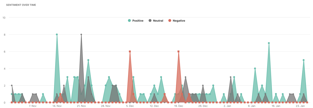
Later in the paper we will discuss in more detail these data and findings. For now, please note that by far the most common application of sentiment analysis has relied on aggregated analyses of the content of document term matrices. In some fewer instances, these analyses may have included changes over time. For an example of how time is traditionally incorporated in SEA, let us look at an output presented by determ, one of the for-profit software tools we mentioned earlier in the “Current applications” section. This output, published in January of 2023, can be accessed at https://cutt.ly/fwlZUgdA. There, analysts at determ showed how sentiments (classified in negative, neutral, and positive), changed from late October to late January (note that no year was specified in this determ’s example).
Although a temporal analysis is useful, for it allows us to observe positive and negative peak changes over this time frame, an even more nuanced understanding of these patterns may be attained by incorporating electors’ individual attributes, like those shown in Figure 5(b). That is, it may be useful to know if the negative peaks observed on December 5th in that determ figure, were driven by electors from specific demographics—women voters, for example. From this perspective, we argue that with a more nuanced level of analyses, better decisions or plans of action may be implemented. For example, if spikes in negative sentiments were driven by women, a campaign may be designed to address their concerns, or with this information we may decide to gather more data (i.e., focus groups or interviews) to better understand the concerns of this group. Accordingly, although disaggregated and group SEA analyses have remained underused, they may deepen our understandings not only in marketing settings (Kennedy & Inkpen, 2006; Taboada, 2016; Turney, 2002) but also in academic and education research (Calvo & D’Mello, 2010; Dolianiti et al., 2018; Luo et al., 2015; Yu et al., 2018; Yu et al., 2016). These analyses, however, although important, do require specialized statistical and computer programming knowledge that has prevented their use among qualitative and mixed methods researchers. Accordingly, a notable contribution of our proposed analytic framework and software is that they were designed to purposefully account for participants’ attributes when conducting the sentiment and emotion analytic procedures without requiring any programming experience.
Attributes in Documents Using Meta Data
Each of the documents uploaded to SENA will be analyzed to detect the distribution of sentiments and emotions in its content. If we decide to add attributes at the document name level, SENA will automatically detect these attributes and will conduct analyses to test whether the distribution of emotions varies across each of the groups. Building from our example shown in Figure 5, let us assume we have two groups, one contains the texts of women and the second of men. SENA will compare the distribution of their emotions via quadratic assignment procedures (more on this below). If we had another group indicating “other,” for example, then the distributions will be compared as women versus men, women versus other, and men versus other, so that we complete all possible pairs of comparisons, which is also referred to as dyadic comparisons.
Dyadic comparisons consist of comparing each of the resulting groups, two at the time. That is, if we have two groups of interest, there will be one statistical QAP test correlation to be conducted (i.e., group 1 vs. group 2); with three groups, there will be three QAP tests (i.e., group 1 vs. group 2, group 1 vs. group 3, and group 2 vs. group 3); with four groups there will be six QAP tests, and so on. In other words, the SENA software has been programmed to apply a combination equation where the statistical tests will be comparing two groups at a time (i.e., dyadic comparisons). This combination equation takes the following form
Panel A in Figure 3 shows the rationale followed to make these comparisons in SENA. In this figure we only have two categories, men and women. To achieve the dyadic analyses, we only need to name the documents based on the attributes of interest and add a number at the end of the file name to differentiate these names. However, if we do not want to conduct comparative analyses, each document name may be different or may only contain one category, as we further illustrate below.
In Panel A in Figure 3 we are showing that each document could have had a different name during data collection. For example, we present a file called “Case 1 in site 2” that is the original file name, but if we intended to add categories, we could add gender attribute by renaming it to “man1.” The second file called “Interview 3, site 3.” should then be named “man2” to account for the category “man.” In the case of women, we also present the original and modified names. The document naming based on attributes is case sensitive. That is, if we have woman3 and Woman4, SENA will consider the latter as another attribute thus resulting in a different category for analysis. We strongly recommend keeping track of these name changes. Note that in Panel C in Figure 3, we also mention that we could add more than one attribute. For example, if we aimed to add ethnicity to this example, in addition to gender, we could then name files: hispanic_man1, black_woman1, black_woman2, hispanic_man2, for example and SENA will conduct all corresponding groups analyses.
In the datasets we are providing for replication, document names that do not include attributes are all called ID
From Figure 3 we can also see that individual level analyses of distributions of sentiments and emotions are also possible as part of this analytic process. That is, one of the outputs presented by SENA, which involves the use of network visualizations, resembles Panel A in Figure 3. In this output, the strength of these participants’ and emotions’ relationships is also captured. These results are particularly relevant when analyses involve participants’ class evaluations as described in our literature review (see Calvo & D’Mello, 2010; Dolianiti et al., 2018; Luo et al., 2015; Yu et al., 2018; Yu et al., 2016). Based on the potential usefulness of SENA for this education-based task, the datasets we are providing include the perspectives provided by students of a data science course, in the form of short essays regarding such a course.
Attributes as a Column in a Database
Panel B in Figure 3 represents how attributes of participants may also be included in databases. This representation is more conventional of quantitative datasets for texts in these data formats are stored in cells (i.e., the intersection of a row and a column). In this format, rows may represent different individuals or the same individuals with different text contributions—over time, for example. In Panel B we show, for example, that Man in the first row provided Text 1, and illustrate that, as part of the analyses, SENA identified “Anticipation” as one of the emotions present in that text. This is important because our databases do not include emotions, instead it is the goal of SENA to apply the lexicons to the text columns and identify those emotions and sentiments.
Following the example shown in Panel A in Figure 3, the attribute of interest in our example shown in Panel B is gender, wherein for consistency (and simplicity) purposes only includes two categories. Note that this decision is entirely up to the research team for, as long as those categories are consistently written (i.e., these categories are case sensitive as well, so if we write Woman and woman, these would be two distinct groups rather than only one), SENA will identify groups as indicated in Panel C in the same figure.
The datasets we are providing cover these three case scenarios described here (i.e., word documents with and without categories, and a dataset). In the first case, we provide access to one corpus configured by 99 word documents with gender categories—available here https://cutt.ly/aeJfFbZt, the second case is a corpus that also contains the same 99 word documents but without these categories—available here https://cutt.ly/leJfF4RW. Finally, the third corpus is stored in an excel spreadsheet with three columns and 99 rows—each of these rows contains one of the essays stored in their Microsoft Word format versions. In this spreadsheet, the first column is the ID, which matches the order of the word documents without categories. The second column contains essays, and the third column contains the gender attributes. For clarity note that this database, available here https://cutt.ly/zeJfHr0M, completely matches the word document essays. As explained in our application section, if SENA users want to account for attributes, they simply need to select the gender column, and SENA will conduct group analyses.
Emotional Entropy or Mixed Messages
Although the identification of sentiments and emotions is reliable based on the lexicon used, there remains the possibility that some texts contain mixed or even contradictory messages. Accordingly, to offer a sense of how prevalent these mixed messaging practices are, all SENA outputs, (i.e., word cloud summaries—see Figure 4—, sentiment and emotion analyses histograms—see Figure 5–, and network analyses—see Figure 6), include a measure of emotional entropy or contradictory messaging, as described next.
Emotional entropy “can be thought of as a measure of unpredictability and surprise based on the consistency or inconsistency of the emotional language contained in a given text. [
Procedurally, emotional entropy is measured as the sum of positive and negative words included in a sentence or text. For example, let us assume we have the following text: “I love hating you and I would be happy if you die.” This sentence has two positive (love and happy) and two negative (hating and die) words. In texts like this example, ties in the number of positive and negative words lead to high emotional entropy values. But as this number of words increases and evenness in the distribution of positive and negative sentiment words decreases, entropy distributions become less extreme. For example, if instead of four words we have 11 and the sentiment distribution is 3 negative and 8 positive, the entropy value would be 0.84. But with the same 11 sentiments, if only one is negative, the entropy is 0.43. When no negative or positive sentiments are mixed with each other, the entropy is zero. These values are obtained from the following two equations

Following Jockers (2015), entropy is standardized to range between 0 and 1 using a Log base 2 or binary logarithm log2 transformation. This transformation is useful because values of 0 mean no change, while negative values indicate reductions and positive values indicate increases. The negative symbol ensures that entropy is always positive. Additionally, it works well with small and long databases. In the emotional entropy value implemented in SENA, every word in the text is counted in the final “sentiment” vector even in the presence of repetitions. That is, if one person used the word “love” three times, this count is represented in “sentiment” as opposed to counting it once, as implemented by Jockers (2015). This change is relevant to our goal of preserving the accuracy of sentiments representation as observed in our participants’ words.
SENA computes entropy values at the text level so that each participant’s text is evaluated following equations (1) and (2). To display individual or text level results, SENA relies on its network interactive visualization. As shown in Figure 6 when we click over an individual (i.e., blue node), a message box displays the estimated emotional entropy of the text that such an individual provided. This same dialogue box displays the proportion of words per participant that were associated with positive sentiments as another tool to understand the mechanisms of each participant’s textual contributions.
Additionally, SENA also offers the average emotional entropy by group when presenting the distribution of sentiments and emotions and the summaries of most frequently used words. Specifically, each title of Figure 4 contains the average entropy of the groups represented in each word cloud. Finally, the average entropy values across all texts, irrespective of groups, is shown in the X-axis of the sentiment and emotion histograms, as shown in Figure 5.
For convenience, each of these values, at both individual and group levels, indicate whether the entropy is considered low, mid, or high. Since the entropy ranges between 0 and 1, we relied on tertiles to capture these values. Specifically, the messages displayed are: “High entropy, high inconsistency” with values greater than 0.66. “Mid entropy, lower consistency” with values over 33 and below 67, and “Low entropy, high consistency” with values below 34.
Pragmatically, we offer emotional entropy estimates with the goal of identifying texts that deserve more attention. For example, if NLP missed sarcasm or the content is more complex by nature, involving a variety of sentiments, thus texts should be more carefully analyzed. Accordingly, by identifying these texts we can qualitatively assess whether the sentiment and emotions analyses were able to capture that complexity or sarcasm or whether we should be concerned with the resulting classification.
Network Modeling and Data Transformations
As discussed above, SENA relies on network analysis methods or relational thinking to identify each unit’s connection strength with the sentiments and emotions embedded in their textual contributions. These relationships are conceptually shown in Figure 3 and are operationalized in Figure 6. Procedurally, recall that each text is analyzed to detect sentiments and emotions, and this process may be represented as a matrix, wherein the rows contain units (i.e., text providers) and the columns are the sentiments and emotions identified across those texts. In returning to our working example, since we have 99 essays, after the sentiment and emotion identification we would have a matrix of 99 rows and 10 columns—with eight of these columns accounting for the emotions discussed above and two columns containing positive or negative sentiments (or polarity).
In sentiment and emotion analyses (SEA) the number of columns will always be 10. This is based on our NRC lexicon use containing eight emotions and two sentiments. From this view, if our total number of texts to be analyzed is 99 and we ignore participants’ attributes, the resulting relational matrix will have 99 rows and 10 columns as its dimensions. From now on, we will be representing these dimensions as [99
In network modeling these matrices are referred to as bipartite or two-mode matrices (Breiger, 1974; González Canché, 2019, 2023, 2024; González Canché et al., 2025b; González Canché & Zhang, 2025a; Kolaczyk & Csárdi, 2014) for they allow us to capture relationships taking place among two types of elements—i.e., the sentiments and emotions embedded in those texts. With these matrices we can add the relational or network attribute to SEA. making it SENA. This is how SENA enables us to build sociograms or network representations like those shown in Figure 6. In these networks the intersection of a row and a column captures the strength of that relationship with true values. That is, if row 88 and column 8 have a value of 24, this means that for this individual’s speech, or text, the emotion contained in column 8 appeared 24 times in her essay or any type of written information. But if this value is zero, this means that such an emotion was not present. The resulting interactive visualizations (see https://cutt.ly/QeJfNb9t and https://cutt.ly/DeJfNILc for Figure 6(a) and (b), respectively) contain this information so that when we place the cursor on top of a connecting line or link, the message box displays the intensity or the number of times that individual mentioned words classified as that emotion. In this network representation, absence of a line indicates that such an individual did not mention words classified under that particular emotion.
As described earlier, the matrices obtained from the NRC lexicon contain both sentiment and emotions. Note further that sentiments reflect polarity with negative and positive categories. That is, in NRC the sentiments are not measured on the same scale as emotions (Jockers, 2015, 2023; Mohammad & Turney, 2013b). Based on this discrepancy in measurement, our network representations along with the quadratic assignment procedures discussed in the following section do not include sentiments but focus on emotions distributions. Having noted this, we are not discarding the distribution of sentiments at the individual level. Instead, we are displaying positive sentiment prevalence in the network visualizations as an attribute of the participants. Specifically, we show an estimate of the proportion of sentiments per actor that were classified as positive—which, as discussed in equation (1), is one of the steps followed to compute the emotional entropy estimates. For example, in Figure 6(a) we can see that a dialogue box shows that for ID8, 80% of his words located in the sentiments lexicon were classified as positive. In Figure 6(b), for participant ID61, 91.7% of her words located in the NRC lexicon were also positive. In addition to this individual level depiction, we also include sentiment distribution in the histograms of sentiments and emotions as shown in Figure 5.
In terms of data transformations, the main implications of focusing on emotions for the visualization and the hypothesis testing via quadratic assignment procedures (QAP) is that the two-mode matrices will be [
Before moving to the next section let us note that our network visualizations weight the size of the emotions via betweenness centrality. Centrality in network modeling serves to highlight the relevance of the actors or units in a network based on their role (Borgatti, 2006; González Canché, 2019, 2023c; Kolaczyk & Csárdi, 2014). Our selection of betweenness centrality is based on our interest in highlighting the emotions that connected more actors in the network or served as bridges. In this centrality, a unit is relevant to the extent such a unit falls in between two other units (Borgatti, 2006; González Canché, 2019; Kolaczyk & Csárdi, 2014). That is, emotions that are connecting or bringing together actors or texts have a bigger size. In the case of men, this emotion was fear (in green) and for women it was trust in purple (see Figure 6(a) and (b), respectively). From this view, our emphasis on these visualizations is to highlight emotions’ relevance while at the same time identifying clusters of cases that are more similar by being connected to the same emotions. That is, units that are located close to each other (blue dots in the figures) tended to mention the same emotions and with a similar intensity than units that are located further away, as we further discuss in our findings section.
Hypothesis Testing via Quadratic Assignment Procedures
When group information is added to texts, SENA automatically tests the hypothesis that some groups’ emotions are more similar than others as a function of the participants’ attributes. For example, in Panel 3 of Figure 3, women seemed to have had more positive emotions than their men counterparts by being ascribed more frequently to surprise and joy, whereas men’s texts were the only ones associated with fear. Although qualitative descriptions like these are important, such descriptions do not allow us to test whether these results are more robust than chance alone. To better understand whether the SENA outputs we observe may present differences by groups, SENA relies on Quadratic Assignment Procedures (QAP), as discussed next.
QAP is a non-parametric analytic procedure that does not rely on normality assumptions and does not assume independence (Krackhardt, 1988). Indeed, QAP “builds into the test statistic the kind of row/column interdependence that is assumed in network data” (Krackhardt, 1988, p. 363). Accordingly, given that QAP enables testing for statistical significance using network data in matrix form (Whitbred, 2011), it is particularly well-suited to help us test “the null hypothesis that two network variables are uncorrelated” (Krackhardt, 1988, p. 362).
As mentioned in the “Network Modeling and Data Transformations” subsection above, this matrix form is obtained from identifying the emotions associated with each of the texts configuring the corpus. We further elaborate on network projections via matrix algebra below. For now, let us mention that QAP takes the form of correlation and regression analyses. In correlation analyses, one can measure the extent to which two networks are statistically associated without any assumption of directionality in this relationship. In regression models directionality exists, and an outcome matrix is explained by a set of network attributes also measured in matrix form to account for all dyadic relationships (Krackhardt, 1988). In both cases, i.e., correlation and regression, QAP translates into measuring whether every corresponding dyad or pair of connections in two (or more) matrices tend to vary in the same direction (positive correlation or association), the opposite direction (negative correlation or association), or whether they are independent.
Procedurally speaking, QAP can be classified under the random permutation test family, which is sometimes referred to as a randomization test (Phipson & Smyth, 2010; Rubin & González Canché, 2019). The random permutation tests begin by recording a given statistic of interest across two mutually exclusive and exhaustive groups. As just discussed above, these statistics can be mean differences, and correlation and regression coefficients, for example. These observed estimates are recorded and then the actual values across these groups are shuffled randomly
In using a correlation coefficient, for example, we could estimate what is the proportion of times that the randomly generated correlation coefficient among two networks was larger than the correlation obtained with the observed data. Once more, the fundamental rationale is that randomly obtained coefficients should be distributed around zero, on average. Hence, if this randomly generated coefficient exceeds the actual observed coefficient, then one would conclude that our observed correlation was not better than what one would expect to see by chance alone. If the proportion of times that randomly generated correlations coefficients are greater in magnitude than our coefficient obtained with actual data approximates zero, then one can conclude that our observed correlations are better than chance by 1 minus the proportion of times randomly generated coefficients were greater. Specifically. assume that .005 is the proportion of times out of 50,000 permutations that the random coefficients surpassed the magnitude of our observed coefficients. Then we can conclude that 99.5% of the times we would expect our observed results to hold true had we had access to other networks of the same size and come from the same population of interest.
Illustration of the Analytic Process and Rationale Employed by the Quadratic Assignment Procedure Analyses.

Matrix Projections
The matrices built from qualitative data analyzed by SENA are the one-mode representation of the actors and their ascription to emotions as represented in Figure 3. This one mode transformation is achieved by network projections as shown in equation (3) (see Breiger, 1974). As described above, the dimensions of the SENA matrices are rows accounting for the number of participants or texts (i.e., 50 rows and 49 rows for men and women, respectively) and the columns are the emotions to which their texts were classified.
In the case of men, the matrix are [50
The element
When the presence of attributes is included in the texts uploaded to the user interface, SENA automatically produces a PDF containing all dyadic comparisons. For example, Figure 7 shows the results of comparing the distribution of emotions contained in the responses provided by women and men at the end of course evaluation of a data science course. The output produced by SENA shows the comparisons conducted, which in this case it reads “Comparisons: man and woman.” Then it shows the statistics of interest. Specifically, SENA prints the observed correlation coefficient Rho in a blue dotted line and a density distribution based on 50,000 permutations. The value of zero is the average correlation across these permutations. The red lines are two standard deviations from the mean obtained from 50,000 permutations. Notably, when the blue line falls in between the red lines, this indicates that the distribution of emotions across these groups is different—that is the matrices are not statistically correlated. Therefore, when the blue line falls outside the red lines, the conclusions are that both groups have emotions that are more similar than chance alone, so there are no significant discrepancies in these distributions.
SENA’s User Interface
SENA’s user interface (UI) is available for Mac (access here: https://cutt.ly/QwhYruBr) and Windows (access here https://cutt.ly/YwhJJKvO) operating systems. As shown in Figure 8, this UI has a maximum of seven steps. The eighth step is optional in case users need to reset the application or change the data format. SENA’s User Interface. Available in Mac (access here: https://cutt.ly/QwhYruBr) and Windows (access here https://cutt.ly/YwhJJKvO) operating systems.
First Step: Data Format Selection
In the first step users need to select word documents (*.doc) or a comma separated value (*.csv) spreadsheet. After this selection, step two will ask users to locate their databases according to the selection made in step one. If the word documents option was selected, users can go to the folder where those documents are stored and select all the documents to be included in the analyses. SENA is programmed to only detect *.doc documents. That is, if the folder selected has multiple document formats, and we select all, only *.doc document will be uploaded to SENA. Note that multiple *.doc files may be uploaded at once, but all these files need to be stored in the same containing folder. If attributes in the names are included, the results will mirror Panel B in Figure 9. If not, they will resemble Panel A in the same figure. Options and results of selecting such options in SENA.
If the option *.csv file was selected, users also need to locate this file. In this case only one file can be uploaded at the time. Note that, as shown in Panel C in Figure 9, once a dataset is loaded, the resulting database is displayed in the UI. After this uploading process is completed, users need to select the columns of interest. After all data are loaded and in the case of the *.csv files and ID, text, and attribute columns are selected, SENA displays the frequencies of all comparison groups. If no attributes were selected, SENA displays the frequencies of all the texts to be analyzed. Due to differences in word document and spreadsheet files, the following subsection elaborates further on these steps, paying close attention to the inclusion of attributes.
Second Step: Aggregate or Disaggregate Analyses Decisions
Figure 9 contains three panels. Panel A shows the output displayed when uploading documents without attributes. As can be seen in this panel, the results display the number of files uploaded and then a table of group distributions indicates that all analyses will be aggregated under the Category ID. As briefly noted above, if every file would have had a different name, instead of displaying “ID,” SENA would have displayed “Aggregate” in the table of groups distributions.
Panel B in Figure 9 shows the same result but in cases when the names of the word documents included gender information. Here we can read this table as indicating that the analyses will contain two groups, and the output includes the frequency of each group.
Finally, Panel C in the same Figure 9 shows the results of loading a database. When a database is loaded, SENA displays the content of this table. Moreover, in this case users need to select whether they want to include a category for comparison or not. By default, SENA selects the option “No_cat_or_time.” This option implies that SENA analyses can also involve temporal elements across participants or may include a combination of attributes across time in the form: “woman_time_1,” “woman_time_2”, for example. If the option “No_cat_or_time” is retained, then the output group distribution table will mirror the word output including only the “Aggregate” categorization. In the case of the essay analyses, we selected the column “Gender,” which translated into the “man” and “woman” categories displayed in Panel C. In the case of the Trump’s comments (more on this dataset below), we selected the option “code” which resulted analyzing texts classified in one of the seven classes learned via machine driven text classification—as we elaborate further in the datasets section below. Finally, note that to formalize the columns selection, SENA requests users to “Execute Columns Selection.” After this execution, a table indicating the number of texts per class or category (i.e., gender and topics in our examples) is displayed.
Third, Fourth and Fifth Steps: Natural Language Processing
In the third step users are asked whether they want to lemmatize (default option) or whether they want to continue without lemmatization. Once this selection is done, we can then proceed to conduct the text mining or natural language processing. As part of this text preparation, and as discussed in the “natural language processing and text preparation” subsection, we have included an optional fifth step. In this step, users may decide to remove words that may be too common and therefore add little nuance to our analyses, as we elaborate further next.
In our essay data example, we decided to remove the first four words of the resulting vocabulary. This output is shown on Panel A of Figure 10. There, we can see that these words were datum (freq = 287), science (freq = 176), student (freq = 155), and course (freq = 94). In our case, we deleted these words because they essentially resembled the prompt we used to ask students to write their or essays—this prompt is shown in the “Short Essays Examples” subsection below. To remove these words in SENA we just need to type their position in the fifth step. Specifically, since these words were the first 4 most frequent words in our vocabulary to exclude them we typed “1, 2, 3, 4” without quotation marks. Let us assume that in other cases the 12th word would also need to be removed. In this case we achieve this by typing “1, 2, 3, 4, 12” also without quotations. After typing these numbers, we click on “Trim Common Words” and the result is shown in Panel B also in Figure 10. Replication data. All links provide full access to these textual datasets (access to data shown in (a) here https://cutt.ly/leJfF4RW, (b) here https://cutt.ly/aeJfFbZt, (c) here https://cutt.ly/zeJfHr0M, (d) here https://cutt.ly/ReLN5yH8).
Sixth and Seventh Steps: Lexicon and SENA Execution
In the sixth step we need to select the Lexicon language. As stated above SENA currently includes Lexicons in 17 languages. Following this multilanguage capability, SENA is programmed to remove stopwords in all these 17 languages. However, the SEA analyses
Once this language selection is completed, we can execute SENA as the seventh step. After the “Execute SENA” button is clicked the word clouds, interactive network visualizations, and sentiment and emotion analyses will be displayed as HTML pages. Additionally, after the processes conclude, a message is displayed below the sixth and seventh steps of SENA’s main panel. An example of this message is shown in Panel C of Figure 10. Specifically, here SENA displays that since we included two groups (men and women, as we show in our applications section below), we have 2 word clouds, 2 network visualizations, and one interactive plot including the SEA analyses. Finally, when group information is included, SENA also renders a PDF with all applicable dyadic QAP correlations. To open and save this file, you can find the link below the seventh step bottom in the left panel.
SENA Applications to Small and Big Data
In this section we present two applications of SENA. The first consists of 99 short student evaluations/reactions about an undergraduate data science course offered at the Guangzhou Institute of Science and Technology, in Baiyun District, Guangzhou, China during the summer of 2024. The second dataset consists of 22,995 comments scrapped from YouTube using the R package “vosonSML” by Gertzel et al. (2022). These comments correspond to five videos analyzing the “second-by-second” evolution of Donald J. Trump’s assassination attempt in Butler Pennsylvania on July 13, 2024. 4 This second dataset analyzed serves to demonstrate how SENA may handle big data and may be integrated with existing software to incorporate machine learning text classification—more on this below.
Short Essays Examples
As described above, the 99 essays included in this section are configured by 50 essays wherein students reacted to the prompt:
As part of this data gathering exercise, we obtained participants gender attributes that resulted in 50 men and 49 women. To illustrate SENA’s performance and flexibility, in the following analyses we present all data formats that SENA can handle, separating the following subsections into Microsoft Word and spreadsheet formats including and not including participants’ attributes.
Word Documents Format
Figure 2(a) and (b) show the data formats that we represented in Panel A of Figure 3. Recall that when no participants’ attributes are added to the Word document metadata, the results will only show: one aggregate estimate of SEA (see Figure 5(a)), one aggregate word cloud, and one network visualization. This network visualization allows obtaining individual estimates of emotions, positive sentiment prevalence, and emotional entropy estimates. This Word document data format is shown in Figure 2(a) and access to this database is available at https://cutt.ly/leJfF4RW.
When attributes are included in the Word document, as shown in Figure 2(b), the outcomes match Figure 5(b) with analyses by each of the groups of interest (i.e., men and women in this case) and two word clouds as shown in Figure 4(a) and (b). Additionally, this process will render a network visualization per group, with all individual level estimates discussed earlier (i.e., emotional entropy, prevalence of positive sentiments and intensity with all applicable emotions). Finally, note that the QAP analyses will be automatically computed, allowing users to download all dyadic analyses in a PDF. Access to this database is available at https://cutt.ly/aeJfFbZt.
Database Analyses of Short Essays
Figure 2(c) shows an example of the data structure in a spreadsheet format. This dataset contains the 99 essays described above but this information is stored in a total of three columns. The first column contains the ID information. The second column is the text content, and the third column contains participants’ attributes that can be used to conduct comparative analyses. Access to this database is available at https://cutt.ly/zeJfHr0M.
Note that the SEA procedures do not allow for duplicate IDs the database. In case your dataset has duplicate IDs, an ID differentiation needs to be executed such as including row numbers. Having noted this, analyses that ignore participants attributes need to simply account for the ID and text columns. As in the case of word documents, these analyses will yield aggregate outputs including a SEA analysis as depicted in Figure 5(a), an aggregate word cloud, and one network visualization.
To incorporate groups analyses, users will need to select the column in the dataset that includes group (or temporal) information. In our dataset shown in Figure 2(c), this information is called “Gender” and is located in the third column. As with the case of word documents that include participants’ attributes, the outputs include SEA analyses as shown in Figure 5(b), two word clouds as shown in Figure 4(a) and (b), network visualizations per group shown in Figure 6 and, and the QAP results compiled in a PDF shown in Figure 7(a).
Application to Machine Learned Classes of Big Data
As briefly described above, the YouTube comments database can be analyzed by video source, that is using each posting account as an attribute and then analyze whether there are sentiments variations these accounts (i.e., the New York Times, The Wall Street Journal, Channel 4 News in the UK, as well two individual accounts). Alternatively, this database can also be analyzed in SENA following a different approach that involves machine learning.
Our analytic strategy consisted of merging SENA with machine learning text classification and then analyzing whether the resulting machine-learned topics or classes vary in their distribution of emotions and sentiments. Specifically, we first determined machine-driven text classes via topic modeling as implemented by MDCOR (González Canché, 2023b) and then analyzed whether there exist variations in the distribution of these sentiments and emotions as a function of the machine-learned classes. This approach enabled us to ask whether machine-learned classes are configured by different distributions of sentiments and emotions as well as the level of emotional entropy those classes contain. From this perspective then, SENA may be easily integrated with existing software and with machine learning text classification applications.
Note that a description of the topic modeling via latent Dirichlet allocation is beyond the scope of this paper. For now, let us simply describe that the result of implementing MDCOR with 5000 MCMC/Gibbs resamplings and 500 burn-in samples yielded the following seven topics as the optimal solution of this text classification learning process: V1. Criticism to the video accuracy, V2. Middle East comments/support, V3. Surprise of failure to stop this attempt, V4. Multiple Conspiracy theories, V5. Belief that it was staged, V6. Love and support for Trump, and V7. Laughing in disbelief. For more details about text classification using MDCOR, please read the methodological paper that provides access to the software in Windows and Mac operating systems (see González Canché, 2023b).
Findings
This section is separated into two sub-sections. The first presents the analyses of short essays aggregated and by groups. The second shows the outputs of the classified comments retrieved from YouTube.
Small(er) Data Analyses
In this section we illustrate how aggregated results may be misleading. Specifically, note that Figure 5 contains the aggregate (Figure 5(a)) and the group analyses (Figure 5(b)) of students’ comments. In this case it is clear that only relying on aggregate analyses would have let us to believe that the vast majority of sentiments (about 70% of them) were positive and that this result may apply to all participants in the sample. This latter issue is referred to as aggregation bias (James, 1982), which as depicted earlier may be minimized by conducting analyses across groups (González Canché, 2023a, 2023b).
Before moving forward, let us further describe the content of Figure 5(a). Each SEA figure presents the outputs separated by negative emotions (left panel), positive emotions (center panel), and sentiment distribution (right panel). This output is normalized so that sentiments distributions (i.e., positive and negative) adds to 1. That is, these distributions are represented in proportions. Similarly, the left and center panels together add to 1 for both account for emotions. In other words, the distribution of the eight emotions represented in this figure adds to 1. The result of the sentiments distribution indicates that there were 264 words across all 99 essays (or 30.9%) that were associated with negative sentiments. In terms of emotions, the most prevalent emotion was trust with a 251 representing 22.8% and the least prevalent was disgust with a frequency of 38 (or 3.5%). The interactive visualization displays these values when posing the cursor on top of each bar. In this example we show the proportions described in this paragraph for the trust and disgust emotions.
Following with our example, Figure 5(b) shows the resulting group analyses output. In that figure we can clearly see that women’s responses were more positive than the comments provided by their men counterparts. The interactive visualization (available here https://cutt.ly/leJddzfw) shows that 86.2% of women’s words identified in the Lexicon were classified as positive sentiments. Subgroup emotion analyses reflected that men tended to have more affiliation with anger and disgust emotions, whereas women’s words were associated with trust, joy, and anticipation. As displayed in this figure we also see that women’s trust almost doubled the trust emotion found in men’s texts (29.2% vs. 17.7%).
Although these differences are notable, we still do not know if such distributions are statistically significantly different. This hypothesis was tested automatically by SENA and the results may be found in Figure 7(a). In this QAP output, we had enough evidence to conclude that emotions distributions of women are different than their men counterparts and that, considering the histogram shown in Figure 5(b) the former tended to be more positive than men’s emotions about this data science course. Specifically, the observed matrix correlation had a magnitude of 0.374, which was not far away from the simulated mean of around 0. That is, the distribution of these matrices is uncorrelated. This findings mean that we can describe the distributions shown in Figure 5(b) as being statistically significantly different.
Figure 6(a) and (b) show individual analyses. These figures are particularly useful in situations where the identification of cases with negative or positive emotions may be of relevance, as described in research where students evaluations were used as predictors of subsequent success (see Calvo & D’Mello, 2010; Dolianiti et al., 2018; Luo et al., 2015; Yu et al., 2018; Yu et al., 2016). As mentioned above, each of these cases also contain emotional entropy estimates that indicate mixed messages in text content. Texts with a mix of positive and negative emotions are classified as confusing, whereas others may be clearer by indicating either negative or positive emotions. Once cases of interest are identified, we could go and read the texts of these cases to gain a deeper understanding of their concerns or praises regarding their experiences. Moreover, following network analyses principles, we can observe how subgroups are formed. For instance, in Figure 6(a) and (b) those participants located in the bottom right sections are more related to a specific set of emotions than participants located in the middle of the graph or in the top right section of this sociogram. For women, bottom right location indicated their affiliation with trust, surprise and joy. For men, participants located in the bottom right were associated with anger, fear, and surprise.
Finally, note that more descriptive analyses may be gained with word clouds. Figure 4(a) and (b) in addition to summarizing content relevance, also show average emotional entropy estimates. These estimates suggests that women have half the emotional entropy values on average than men. That is, men’s texts were less clear regarding their inclusion of positive and negative emotions.
Big Data Analyses of Machine-Learned Topics
As mentioned above, the analyses of YouTube comments involved a classification of these comments and then analyzing whether the emotion distribution of those comments were different or similar. Just as in the short essay case, Figure 11(a) shows that an aggregate analyses of the seven topics identified via machine learning could be understood as having more positive sentiments. However, the disaggregate analyses shown in Figure 11(b) suggest that topics 6 and 7 (Love and support for Trump and Laughing in disbelief or nervously, respectively) were associated with more positive sentiments and emotions. Of the other five topics, only topic 1 (Criticism to the video accuracy) was associated with more negative sentiments and emotions than all the other remaining topics. Examples of SENA Outputs Displayed in its User Interface.
Access to all word clouds and SENA outputs per topic may be gained by following this link https://cutt.ly/ieZlGeOI. For this example, let us address the question of whether emotions distributions are similarly distributed across topics. To this end we can use the QAP output. However, given that 7 groups or topics exist, the resulting dyadic combinations rendered 21 comparisons. These comparisons are shown in Figure 7(b).
Overall, these results confirmed that the discrepancies observed in Figure 8(b) are important. All comparisons that included topics 6 and 7 (Love and support for Trump and Laughing in disbelief or nervously, respectively) consistently indicated that the positive emotions captured in these topics were different from those captured in topics 1 to 5. Of these latter topics, topic 1 captured the most negative emotions. But topic 1 (Criticism to the video accuracy) was only significantly different from topic 2 that included Middle East comments/support. Note that when an extremely potentially viral topic exists in social media, groups tend to “profit” from that topic by posting their support to issues that they care. In this case, the issues were then concurrent conflicts in the Middle East. Finally, topics 6 and 7 were highly correlated, therefore allowing us to conclude that they are configured by similar distributions of emotions, which as shown in Figure 11(b) are overwhelmingly positive.
In closing this section, let us note that a study focused on the analyses of these datasets would proceed to qualitative analyzing the most relevant texts. This identification can be done using cases shown in the SENA outputs, either individually or by their location in the resulting sociograms. Specifically, as discussed in Figure 6(a) and (b), certain individuals and groups tend to be clustered together by being linked to similar emotions. This identification of cases could help researcher to qualitatively explain why group differences were found, preferably using participants’ own voices, as captured by their original essays or comments (see González Canché, 2023a, 2023b, for examples of the relevance of preserving these voices).
Discussion, Limitations, and Future Steps
As discussed above, our motivation for integrating sentiment and emotion analyses with qualitative research is that the latter “involves finding out what people think, and how they feel” (Rambocas & Gama, 2013, p. 14). From this perspective, we believe that “[w]hen integrated with qualitative research, sentiment [an emotion] analysis can be used as a tool that promotes […] structure to an otherwise flexible and [perhaps even more] subjective […] data analysis process” (Rambocas & Gama, 2013, p. 15). Accordingly, our study presented an analytic framework and multi-platform software application developed to conduct sentiment and emotion network analyses. This is a contribution to qualitative and mixed-methods literatures because most current applications of sentiment and emotion modeling focus on providing aggregated analyses rather than on allowing for the testing of group variation and individual experiences.
From this brief discussion, a salient contribution of the analytic framework we are proposing consists of offering a statistical test of sentiment changes across groups. Hypothesis testing is another related but different departure from traditional sentiment and emotion analysis because current applications of sentiment and emotion analysis have remained purely descriptive in nature, even in cases when temporal elements have been incorporated (as we discussed in the determ’s example on page 20). This lack of testing on statistical variations is precisely due to the fact that, other than time-based variations, sentiment and emotion analyses frameworks are yet to include participants (or texts’ attributes) that may be used for statistical comparisons. In our analytic framework and software these statistical tests are conducted via quadratic assignment procedures (QAP) correlations, as described above. In sum, we believe that with SENA researchers can comprehensively take advantage of the insights that can be gained with the analyses of
Based on this discussion, let us then summarize that the SENA framework and software contributes to this literature in the following aspects: (1) SENA focuses on the use of sentiment and emotion analyses for academic research, even though the software does not prevent its use for marketing purposes. (2) SENA allows for the incorporation of participants’ texts attributes into the analytic process, in order to gain more nuanced understandings of potential group variation. (a) Moreover, the resulting interactive visualizations will also allow the identification of individual cases (i.e., texts) that showed particularly stronger sentiments and emotions as well as (b) discrepancies or inconsistencies in the presence of positive and negative sentiments and emotions (i.e., emotional entropy) in speeches based on the use of positive and negative emotions (Nandwani & Verma, 2021) at both the individual and group levels. (3) SENA also allows for the statistical dyadic statistical comparison of similarities and differences in emotion distributions across these groups of interest via quadratic assignment procedures (Hubert & Arabie, 1989; Krackardt, 1987). (4) SENA allows all these analyses without the need to develop any statistical or computer programming proficiency, for its development is intended to help democratize access to data science.
SENA aligns with an equal status integrative mixed method design (González Canché, 2023a, 2023b, 2024). That is, once the outputs are produced, qualitative analyses must follow to gain deeper and more nuanced understandings of our participants’ sentiments and emotions on the topic of interest. Similarly, if needed more data may be collected by interviewing individuals identified during the analysis of the SENA outputs, in case this may be helpful in better understanding their experiences.
As discussed above, SEA provides us with time efficient insights into the distribution of positive or negative experiences or opinions (i.e., sentiment analysis) and the range of feelings or emotions (i.e., emotion analysis) expressed by our informants, customers, users, or participants (Nandwani & Verma, 2021). In this respect, and although typically sentiment and emotion analyses are used for profit purposes (i.e., marketing, consumer behaviors and preferences) our discussion focused on the use of SENA in academic settings (i.e., to better understand our research participants’ experiences and opinions) or to understand social phenomena (i.e., the reactions of thousands of YouTube users who posted comments regarding the assassination attempt). We were purposeful in these uses for we hope SENA may become a tool that qualitative and mixed-methods researchers may employ in the analysis of qualitative evidence.
Limitations
SENA currently does not incorporate machine learning and artificial intelligence in the identification of sentiments and emotions. We refrained from this approach because those AI applications cannot yet be computed locally without the use of quite powerful computers. Instead, these AI applications, either need a server connection where our qualitative data needs to be uploaded or super computers to accommodate the large language processing power needed. With respect to the former, given the need to protect participants confidentiality and anonymity in academic research, which is the primary audience for the application of SENA, we preferred to offer access to 17 languages rather than require users to upload their databases to servers. With respect to the computing power costs, even if we develop local servers, costs will still impede the vast majority of qualitative researchers from benefiting from SENA.
Having noted this potential limitation, we also showcase how SENA may be easily incorporated with existing machine learning procedures like those implemented with no-code software like “Latent code identification (LACOID)” and “Machine driven classification of open-ended responses (MDCOR)” (see González Canché, 2023a, 2023b, respectively). In these latter applications, we first need to classify the raw text into codes or topics and then apply SENA to these learned classes to test whether the distribution of emotions is similar or statistically diverges. This analytic flexibility is notable because we can include machine leaning and AI to texts that will then be analyzed via SENA without compromising the integrity of the analyses.
Final Thoughts and Next Steps
The present document focused on the analysis of textual or unstructured data with an emphasis on academic research or on how researchers may benefit from this tool by considering the temporal evolution of emotions or the changes in the distributions of such emotions across groups. Although future iterations of the framework and software we are presenting may more formally include machine learning or AI applications, until personal servers may be easily and affordably implemented, for now and due to privacy and financial cost concerns, we are presenting a natural language processing implementation that runs completely locally and does not require the uploading of any output or data to any server. Having said this, the level of anonymity varies depending on the source. For example, while the YouTube comments do not require any type of confidentiality protection for they are made public when users shared them online, essays data or interview transcripts for example need to be handled with more caution.
In terms of confidentiality protection, note that for the essay database, although we are presenting our interactive outputs online, before doing so we were sure to (a) anonymize all texts, (b) such texts did not include any potential harmful information, (c) we requested written permission from participants, and (d) the online posting of these outputs is completely optional. With respect to the last point, let us note that the use of SENA does not, in any way, imply that the outputs will automatically be made available online; instead, this is an extra step that is completely based on the research team goals, interests, and motivation. This motivation, in our case, was to showcase the interactivity of these outcomes so that the qualitative and mixed-method research community may interact with such online outputs.
Finally, we emphasize that sentiment and emotions analyses’ historical salient concentration on marketing or market research (Nandwani & Verma, 2021; Sharma et al., 2024) can still be implemented with SENA. However, we developed SENA with a particular interest in applying it as a tool to better inform mixed methods and qualitative research. As such, our interest in providing a multi-platform software, along with all data used in this study, aimed to facilitate qualitative and mixed-methods researchers’ firsthand interaction with SENA. We hope this strategy may ease access to data science applications without the need to learn computer and statistical programming, which, aside from monetary costs, arguably remains the most important barrier to benefit from these tools in qualitative and mixed-methods research. This is why we are offering these tools completely free of charge so that no financial barriers exist in its implementation and data science democratization is a step closer to reaching our research communities—for another no-code application, please see González Canché, 2025c.