
Abstract
Keywords
Introduction
Rolling bearings are the core component of rotating machine rotor, which are widely used in wind power, gas turbine, and other fields. For the gas turbine field, rolling bearings work in complex and changeable environments all year round. If the rolling bearing fails, even a slight failure can easily cause the rotor to rub, and cause serious mechanical damage. Due to the different degrees of bearing faults, the symptoms of the faults are also different. Therefore, bearing fault diagnosis has become the research focus of scholars at home and abroad.
According to the rotor dynamics, the vibration signal of the mechanical component can represent the health status of machinery. 1 With the application of vibration signal analysis methods, abundant research achievements have been made in the field of rolling bearing diagnosis. 2 Many scholars collected vibration signals from the laboratory simulation platform, and combine them with wavelet transformation, 3 genetic algorithm (GA), 4 and other algorithms to study fault vibration signals. However, due to the location of the bearings of rotating machinery such as aero-engine, the vibration sensor cannot be directly installed on the bearing seat. Therefore, the vibration signal collected by the sensor installed on the casing has obvious coupling, bearing fault signal is more likely to be overwhelmed by noise.
For the above situation, algorithms such as empirical mode decomposition (EMD), 5 blind source decomposition, 6 variational mode decomposition (VMD) 7 have been applied to the analysis of bearing fault vibration signals, and have achieved fruitful results with the efforts of many scholars.5–7 In the literature, 8 the empirical mode decomposition (EMD) method was used to decompose the vibration signal, and the components were selected according to the energy distribution of the eigenmode components to reconstruct the signal. Then, the time-frequency domain eigenvalues of the reconstructed signal were extracted as the fault data set of the faulty bearing. In the literature, 8 only the time-frequency domain characteristics of the vibration signal were used for fault diagnosis, and the value of the vibration signal component cannot be fully explored. And they did not propose a method to solve the problems of endpoint effect, mode aliasing, over-envelop, and so on in EMD. In the literature, 9 singular value decomposition method was adopted to solve the problem of EMD, but this method leads to the new problem that it was difficult to determine the number of rows and columns of Hankel matrix. In the literature, 10 authors used blind source analysis to analyze engine vibration signals, but blind source separation requires multiple observations, which was difficult for single-channel vibration signal analysis. In the literature, 11 they adopted Hilbert transform method to diagnose bearing faults based on fault features in square envelope. In the literature, 12 the authors used Variational mode decomposition (VMD) to analyze the vibration signal, and used the envelope spectrum eigenfactor automatic search strategy to solve the drawbacks of VMD parameters, so as to realize the early fault diagnosis of bearings. In the literature, 13 the authors used particle swarm optimization (PSO) algorithm to solve the problem of parameter selection in VMD decomposition, and used the singular value energy spectrum of components to judge the health status of bearings. Although the envelope entropy value can reflect the sparsity of the signal, it cannot identify the number of vibration sources in the vibration signal. And the random initialization of the PSO algorithm population will affect the numerical calculation results, and repeated iterative operations will also increase the diagnosis time.
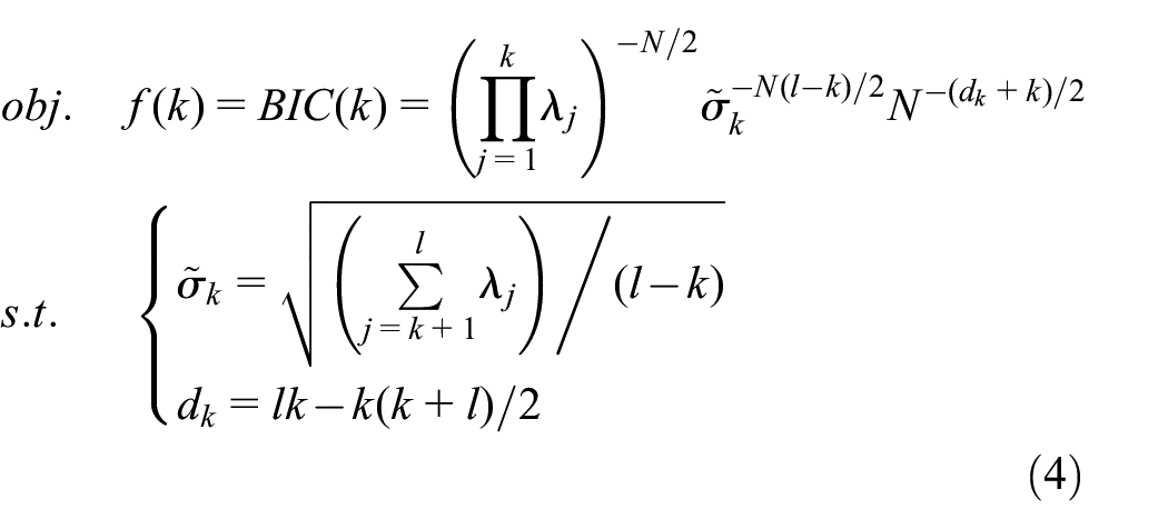
Aiming at the problem that VMD is difficult to determine the number of modal components and the value of the penalty factor, the Bayesian information criterion is used in this paper to estimate the number of vibration sources of the vibration signal. Then the number of vibration sources is brought back to the VMD to decompose the vibration signal again, and the singular value energy of different types and different fault components is extracted as the fault data set.
Support vector machine (SVM) has the advantages of simple structure, high computational efficiency, and few influencing parameters. And SVM can use a small number of samples to solve the problem that it is difficult to distinguish samples in nonlinear high-dimensional space. 14 However, the performance of SVM in classification depends largely on the selection of kernel functions and kernel parameters. At present, the commonly used parameter optimization methods are grid search method, genetic algorithm (GA), and so on. As a stochastic algorithm that utilizes the computer’s high-speed computing ability, the GA has shown considerable effects and is widely used to solve the optimization problems of bearing diagnosis.
Traditional GA refers to genetic properties in biology, including iterative computations such as selection, crossover, and mutation, which might have certain drawbacks, for example, local optimization and premature in solving the highly nonlinear complicated optimization problems. To overcome these drawbacks, an improved genetic algorithm (IGA) was proposed in the literature. 15 Therefore, based on the research results of the literature, 15 this paper proposes an improved support vector machine diagnostic model optimized by IGA. In this paper, based on the sample data set obtained by the VMD algorithm, an optimized support vector machine is used to diagnose bearing faults. The simulation results show that the Bayesian information criterion can accurately identify the number of vibration sources in the vibration signal. The effectiveness of the proposed method is verified by the diagnosis of different bearing faults.
Optimized VMD
Theory of VMD
The goal of VMD is to decompose a real-valued input signal
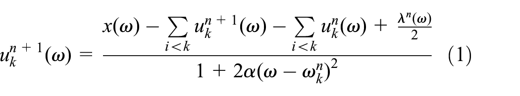
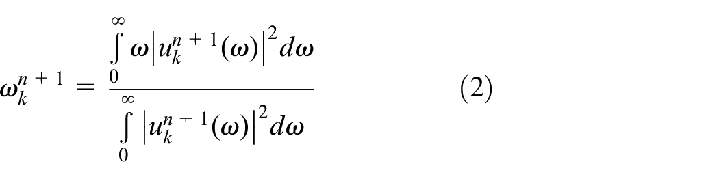
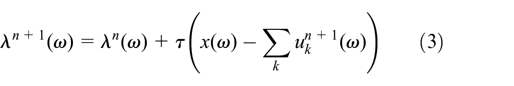
Optimized VMD
Since the number
The vibration signal
Where,
The flow chart of VMD optimized by BIC (VMDBIC) is shown in Figure 1.
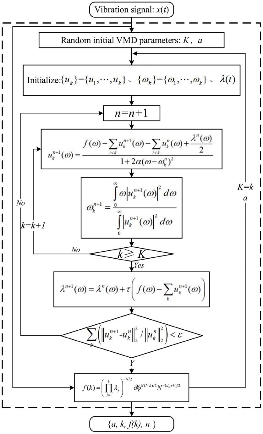
The flowchart of improved VMD.
The number of vibration sources obtained by the same equipment is the same, but the vibration signal components
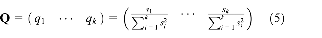
Where,
Algorithm verification
The simulation signal is used to verify the effect of VMDBIC. In the simulation process, the sampling frequency of the vibration signal is 1024 Hz, and the sampling time lasts 1 s. The simulation signal is obtained by the following equation (6):
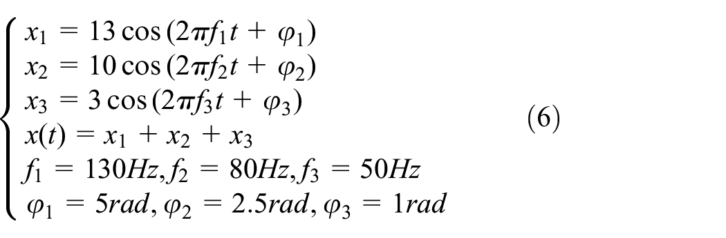
The simulation signal

Time domain and frequency domain diagram of simulation signal.

Time domain and frequency domain diagram of VMD decomposition.
The vibration signal
Eigenvalue of matrix


Time domain and frequency domain diagram of VMDBIC decomposition.
The index of orthogonality (IO) and the index of energy conservation (IEC) are used to further evaluate the decomposition effect of VMDBIC. If the IO value is smaller, it means that the orthogonality of each IMF component is better, and the decomposition precision is higher. 13 If the IEC value is closer to 1, it means that the energy leakage during the decomposition process is less, and the decomposition effect is better. 13 The calculation methods of IO and IEC are shown in equations (7) and (8).
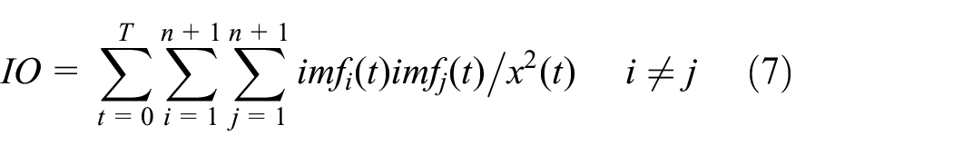
Where,
The IO and IEC calculation results of VMD and VMDBIC algorithms are shown in Table 2. In terms of IO, the calculated value of VMDBIC is 0.0322 lower than that of VMD. In terms of IEC, the calculated value of VMDBIC is 0.0403 higher than that of VMD. Therefore, it can be found from the calculation results that the decomposition effect of VMDBIC on the signal is better than that of VMD.
Comparison table of VMD and VMDBIC.

Optimized SVM
Support Vector Machine (SVM) can transform low-dimensional linearly inseparable problems into linearly separable problems by mapping them to higher-dimensional Spaces.
14
The penalty parameter
What’s the SVM
Suppose that the samples (

Where,
In order to ensure that the optimal classification hyperplane can be calculated in
Where,
Where,
Optimized SVM
The main factors that determine the fault identification ability of the SVM diagnosis model are the penalty parameter
Where,
In equation (15),
Bearing fault diagnosis process
The bearing fault diagnosis process based on VMDBIC and IGA-SVM are shown in Figure 5. The process is mainly composed of four parts, including VMDBIC (

Bearing fault diagnosis process based on VMDBIC and IGA-SVM.
The process is briefly described as follows: Firstly, the vibration signals of bearing faults under different working conditions are collected through the laboratory bearing fault simulation platform. Secondly, BIC is used to optimize the modal number and penalty parameters of VMD. Thirdly the optimized VMD is used to decompose the vibration signal under different working conditions, and the singular value energy spectrum is calculated to construct the fault characteristic sample data. Finally, IGA is used to optimize SVM and the optimized SVM is used for bearing fault diagnosis.
Bearing experiment description
Bearing experiment description
The bearing data used in the research are collected from the bearing test platform of Case Western Reserve University 19 and the author’s unit. The schematic diagram of the bearing test platform is shown in Figure 6.
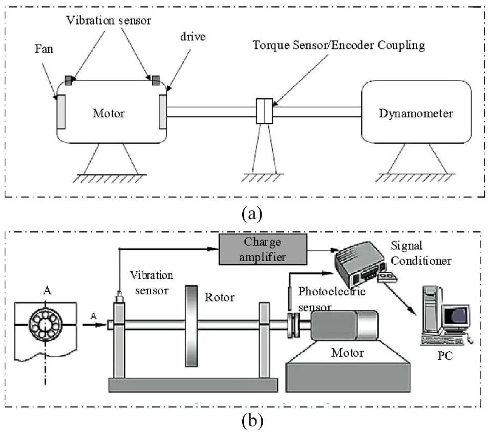
Schematic diagram of the bearing test platform: (a) schematic diagram of bearing test bench at Case Western Reserve University and (b) schematic diagram of laboratory bearing test bench.
In the bearing test platform of the author’s unit, the 307 bearing is used as the research object. In the bearing test platform of Case Western Reserve University, the SKF6205 bearing is used as the research object at the fan end, and the SKF6203 bearing is used as the research object at the drive end. The dimensions of the bearing are shown in Figure 7. The bearing fault size and experimental conditions used in the experiment are shown in Table 3. Under the loads of 0, 0.75, 1.5, and 2.25 KW respectively, the vibration signals of bearings of different types and working conditions are collected from the test platform of Case Western Reserve University. Under the 0 load, the bearing vibration signal is collected from the test platform of the author’s unit.

Schematic diagram of bearing size: (a) 307, (b) SKF6203, and (c) SKF6205.
Different types of bearing fault information.

Data set preparation
In order to facilitate the analysis of the experimental results, each type of fault data is numbered. The numbering rule is: “model + initial letter of working condition + serial number.” Such as “
The vibration signal fault types collected in the experiment are single-type fault data. There are 24 sets of bearing fault condition types in total, and each type of fault type data is 200, with a total of 5600 sets of data.
Since there are 24 sets of bearing vibration signals, the number of vibration sources estimated by the Bayesian information criterion for different vibration signals may be different (the distribution of the number of vibration sources for the 24 sets of vibration signals is shown in Figure 8). In order to ensure the consistency of the vector dimension of the constructed fault feature data set constructed subsequently, considering the distribution of the source number and the actual situation, the number of modal components of the VMD is set to
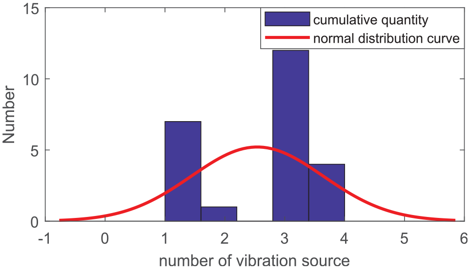
Vibration source number distribution diagram.
Since there are 24 types of bearing failures, considering the length of the article. Therefore, in the description in this paper, the vibration signals of SKF6205-B-1 and SKF6203-B-1 under 0 load are taken as examples to analyze and process them. The vibration signal analysis results of SKF6205-B-1 and SKF6203-B-1 are shown in Figures 9 and 10, respectively. From the time-domain and frequency-domain diagrams, it can be seen that the modal spectrum of each component do not overlap significantly, and each component has a different center frequency band, which shows the effectiveness of the VMDBIC method. Therefore, VMDBIC is used to decompose 24 types of bearing fault types, and the eigenvectors of various faults are calculated according to equation (5).
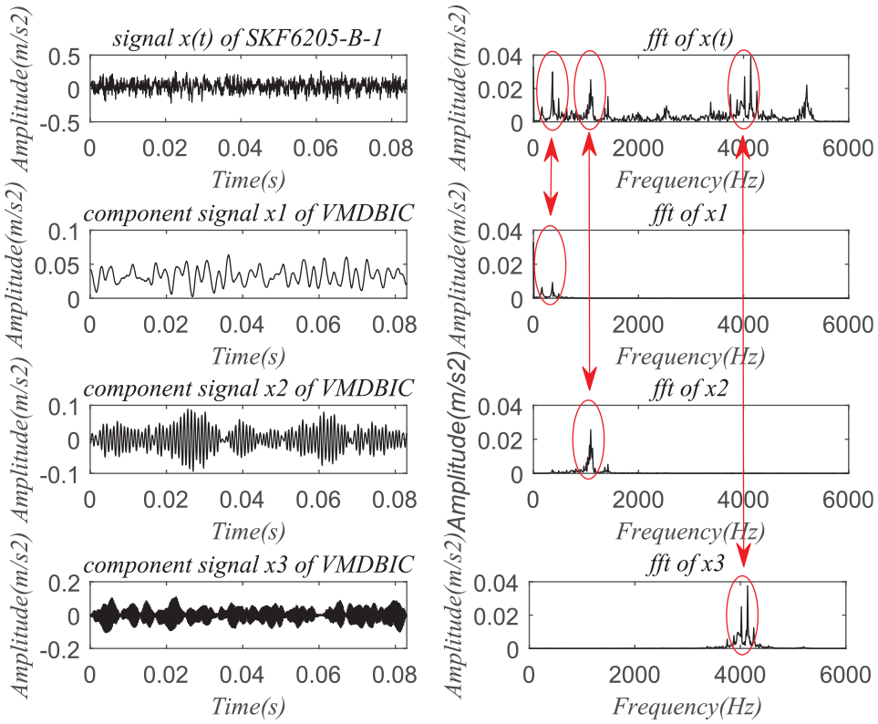
SKF6205-B-1 vibration signal analysis.
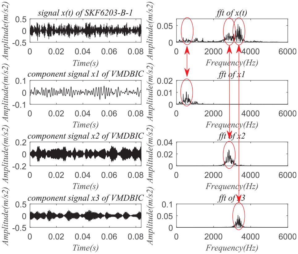
SKF6203-B-1 vibration signal analysis.
Analysis of diagnostic results
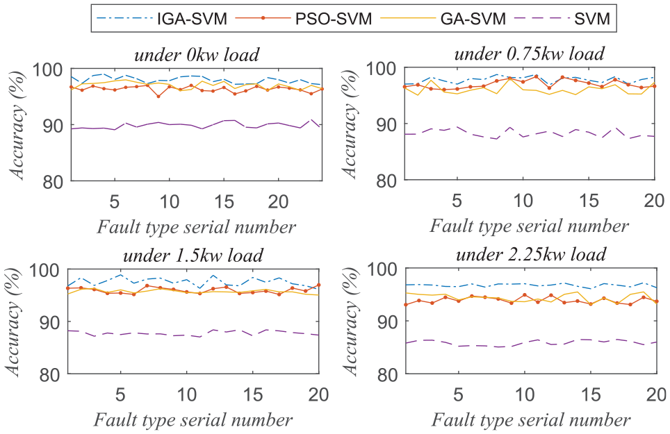
There are 24 sets of bearing fault condition types in total, and each type of fault type data is 200, with a total of 5600 sets of data. 80% of the sample data of each type of fault is used as the training set sample, and 20% is used as the test set sample. In order to verify the effectiveness of the method in the paper, the cross-validated SVM, the classical genetic algorithm (GA) optimized SVM (GA-SVM), and the classical particle swarm optimization (PSO) optimized SVM (PSO-SVM) are used as comparison models. The parameters of the cross-validated SVM uses cross-validation to correct the kernel parameters and penalty parameters. The parameters of GA are the same as IGA, including iteration step is 60, the population size is 10 and its range is [−0.5 0.5], the crossover probability is 0.6, the mutation probability is 0.05, the
Diagnosis accuracy analysis
To avoid the difference in the diagnosis result caused by the inconsistency of the population initialization in the algorithm, so based on the same data set and algorithm, the average value of the repeated diagnosis 30 times is used as the result evaluation standard. The bearing fault samples are diagnosed by several algorithms mentioned in the previous section. And its diagnostic results of several algorithms are shown in Table 4.
Identification of fault conditions by the diagnosis model.

It can be seen from Table 4 that the recognition accuracy of IGA-SVM, PSO-SVM, and GA-SVM diagnostic models for different bearing fault conditions all reach more than 90%. In contrast, the diagnostic performance of cross-validated SVM is poor, which indicates the necessity of SVM optimization. In order to compare the diagnostic results of several diagnostic models more intuitively, the results in Table 4 are visualized as Figures 11 and 12. The fault diagnosis results of different loads are shown in Figure 10 (the abscissa number in the figure represents the fault type in Table 4). In Figure 12, the average value of the diagnosis results of each fault condition under load power is used as a criterion to compare the fault identification effects of each diagnosis model under different loads. It can be seen from Figures 11 and 12 that under the loads of 0, 1.5, and 2.25 KW, the diagnosis effect of IGA-SVM is obviously better than other diagnosis models. However, under the load of 0.75 KW, the diagnosis results of IGA-SVM for some fault types are similar to those of other models, which may be caused by the different sensitivity of some fault types to the load.
Identification of fault conditions by the diagnosis model.
Average fault recognition rate.
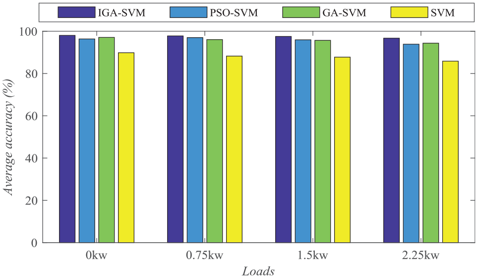
Analysis of diagnostic results under different loads
Although the fault identification rates of several diagnostic models under different loads are listed in Table 4, it cannot directly show the impact of load changes on the accuracy of fault diagnosis. Therefore, the average value of the diagnosis results of each fault condition under different load powers is used as the standard to analyze the influence of load changes on the diagnosis model. It should be noted that since the laboratory bearing data are obtained under 0 KW load, the laboratory bearing data are not included in the analysis at this stage. The effect of load change on the diagnostic model is shown in Figure 13. It can be seen from Figure 13 that the effect of load changes on several diagnostic models is relatively small, which may be because the extracted fault feature sample data can accurately reflect the fault information.
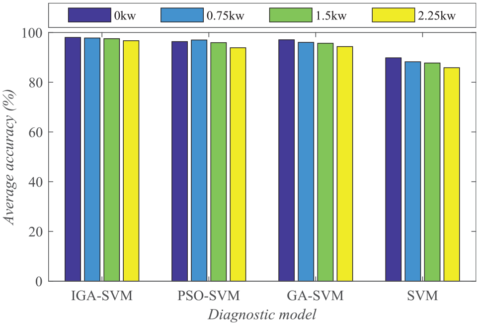
Influence of load variation on recognition rate.
Mutual diagnosis analysis of different types of bearings
When the load power is 0, the mutual diagnosis of different types of bearing faults is studied. That is, use the sample data of bearing A to train the diagnosis model, and then use the model to diagnose the sample of bearing B. In order to ensure the effectiveness of bearing fault diagnosis, select samples with similar bearing fault sizes, including SKF6205-I-3, SKF6203-I-3, 307-I-4, SKF6205-O-1, SKF6203-O-1, 307-O-5, SKF6205-B-1, SKF6203-B-1, 307-B-5. There are two types of scheme design: one kind of bearing diagnoses two kinds of bearings, and two kinds of bearings diagnose one kind of bearing. The detailed scheme is shown in Table 5 (In Table 5, “√” indicates the bearing type used for training set or test set). In the experiment, all the fault data of the selected bearing are used as the data members of the training set or the test set, and there is no phenomenon that the same bearing data is divided into the training set and the test set.
The experimental scheme.

In addition, in the experiment, the diagnostic model only adopts the IGA-SVM model. To avoid the difference in the diagnosis result caused by the inconsistency of the population initialization in the algorithm, so based on the same data set and algorithm, the average value of the repeated diagnosis 15 times is used as the result evaluation standard. And the diagnostic results of IGA-SVM is shown in Table 6. It can be seen from Table 6 that the effect of mutual diagnosis between different types of bearings is poor. But after careful analysis of Table 6, it can be found that the diagnostic effect of scheme 6 and scheme 1 is better than that of other schemes. It can be found from Figure 7 that due to the obvious difference in the dimensions of the three bearings, there are obvious differences in the frequency doubling of the bearing fault characteristics. The bearing fault sample data is obtained by decomposing the vibration signal by VMDBIC and calculating according to equation (5). Among them, the components of VMDBIC have different center frequencies, and these center frequencies are implicitly representative of the fault characteristic frequency doubling. The diagnostic results of schemes 2–5 show that the training set samples have little significance for the learning of the diagnostic model. The characteristics of the fault samples are highly discrete, which makes the diagnosis model unable to capture the corresponding characteristics. The diagnosis effect of scheme 6 is better because the fault frequency of SKF6205 bearing is between SKF6203 and 307, and the model can learn some characteristic information.
Fault identification accuracy.

Conclusion
In order to solve the problems of high noise of bearing vibration signal, uncertain vibration source and low fault identification rate, this paper proposes the variational modal decomposition method optimized by Bayesian information criterion and the fault diagnosis method of SVM optimized by improved genetic algorithm.
Firstly, VMD is used to decompose the vibration signal, and Bayesian information criterion is used to estimate the number of vibration sources of the vibration signal. Then the number of vibration sources is taken as the number of components of VMD, and decompose the vibration signal. The simulation results show that the effectiveness of the method is proved from the time-domain, frequency-domain, orthogonality index and energy conservation index of the decomposed signal. Since there are 3 bearing types and 24 fault types in this paper, the VMDBIC method will obtain different vibration source numbers when decomposing different fault types. Therefore, the value of the modal component of the VMDBIC model is determined by analyzing the distribution of the number of vibration sources of each vibration signal, so as to construct the characteristic variables with the same dimension.
The SVM model optimized by the improved genetic algorithm is used in the bearing fault diagnosis example. The accuracy of the IGA-SVM diagnosis model for 24 kinds of faults is higher than that of other comparison models, and its load change has little impact on the diagnosis effect of the model. In this paper, six schemes are designed to study the mutual diagnosis of different types of bearing faults. The analysis results show that the fault characteristic frequency of the bearing has an obvious influence on the mutual diagnosis between the bearings. In order to establish a diagnostic model that can adapt to various types of bearings, further research and analysis are required.