Sage Journals: Discover world-class research

Abstract

Real-time traffic control is very important for urban transportation systems. Due to conflicts among different optimization objectives, the existing multi-objective models often convert into single-objective problems through weighted sum method. To obtain real-time signal parameters and evaluation indices, this article puts forward a Pareto front–based multi-objective traffic signal control model using particle swarm optimization algorithm. The article first formulates a control model for intersections based on detected real-time link volumes, with minimum delay time, minimum number of stops, and maximum effective capacity as three objectives. Moreover, this article designs a step-by-step particle swarm optimization algorithm based on Pareto front for solution. Pareto dominance relation and density distance are employed for ranking, tournament selection is used to select and weed out particles, and Pareto front for the signal timing plan is then obtained, including time-varying cycle length and split. Finally, based on actual survey data, scenario analyses determine the optimal parameters of the particle swarm algorithm, comparisons with the current situation and existing models demonstrate the excellent performances, and the experiments incorporating outliers in the input data or total failure of detectors further prove the robustness. Generally, the proposed methodology is effective and robust enough for real-time traffic signal control.

Keywords

Pareto front signal control multi-objective optimization particle swarm

Introduction

Real-time traffic signal control is very important for operation and management of urban transportation systems. During the past several decades, many models have been developed to optimize real-time signal timing parameters, and they can be mainly divided into two groups: mathematical programming method and simulation-based approach.

Most mathematical programming models are formulated based on the interrelations between evaluation indices (delay time, number of stops, queue length, capacity, etc.) and signal parameters (cycle, split, offset, etc.). They focus on seeking timing plan to optimize single or multiple objectives and to satisfy real-time traffic flows. During rather long evolution process, many researches have devoted to oversaturated traffic condition, which is more valuable for practical transportation systems. In pioneering works, minimum delay time has been taken as the optimization objective.^1–3 Michalopoulos and Stephanopoulos^4–6 further introduced the queue length constraints into intersection control and took the spillback phenomenon into account. Moreover, Ahn and Machemehl⁷ integrated two objectives into the signal timing in oversaturated arterial networks: to maximize the number of passed vehicles and to minimize the queue spillback occurrence. All the above objectives have been used widely in traffic signal control in the literature.

Recently, multi-objective traffic control models have been studied extensively due to their good performances. Lieberman et al.⁸ formulated a real-time control model for oversaturated arterials, with three objectives, that is, to maximize system throughput, to fully use storage capacity, and to provide equitable service. Ceder and Reshetnik⁹ put forward two signal models for undersaturated and oversaturated intersection, respectively, with minimization of maximum queue and accumulative queue as the two objectives. Talmor and Mahalel¹⁰ further introduced the maximum capacity into the objectives of signal control and presented an algorithm for signal design of an isolated intersection during congestion.

Many multi-objective traffic control models have been transformed to single-objective problems using weighted sum method, for instance, Jiao and Sun¹¹ proposed a multi-objective optimization model to minimize delay time and queue length and to maximize effective capacity and converted the original model into a single-objective problem through three weight coefficients. Meanwhile, some scholars solved the non-inferior solution problems based on Pareto front or fuzzy control methods. Schmöcker et al.¹² developed a multi-objective signal control model for urban junctions and employed fuzzy logic where the membership functions were optimized using the Bellman–Zadeh principle of fuzzy decision-making. Case studies indicated that it led to a Pareto-optimal solution directly, and different objectives could be balanced easily by setting their acceptability and unacceptability thresholds. Shou and Xu¹³ used fuzzy control method to minimize delay time, number of stops, and queue length simultaneously for oversaturated intersections. The existing researches have proved that the combination of different objectives led to unfair competitions among evaluation indices, and non-inferior solutions of multi-objective control could realize the general optimization, despite the rather difficult algorithm.

Based on the existing mathematical programming models, some simulation-based approaches have been developed integrating traffic flow interactions. One of the representatives of early simulation-based methods is Traffic Network Study Tool (TRANSYT) described in Robertson,¹⁴ Wallace et al.,¹⁵ and Wong.¹⁶ Incorporating time-varying traffic information, some real-time adaptive traffic control systems were further developed, which were also simulation-based approaches, such as Sydney Coordinated Adaptive Traffic System (SCATS),^17,18 Optimized Policies for Adaptive Control (OPAC),¹⁹ Split, Cycle and Offset Optimization Technique (SCOOT),^20,21 Real-time Hierarchical Optimized Distributed and Effective System (RHODES),²² and so forth. All the above simulation-based approaches have been applied in practical traffic control all over the world; however, most of them are not applicable to Chinese cities, due to the complex mixed traffic flow conditions.

Unquestionably, time-dependent turning movement flows are very important input data for traffic signal control at intersections; however, they were unavailable from the existing traffic surveillance systems. Fortunately, such turning flows could be estimated using dynamic origin–destination estimation methods, such as Jiao et al.^23–26 Therefore, we can employ time-varying turning flows as the input data and formulate the multi-objective real-time traffic signal control models for intersections. Furthermore, traffic parameters based on prediction are also very important for traffic control, which have also been considered in several researches.^27–29

Since solution of nonlinear problem is not straightforward, some heuristic algorithms and swarm intelligence–based algorithms have been developed, for example, genetic algorithm (GA), ant colony optimization (ACO) algorithm, and particle swarm optimization (PSO) algorithm. PSO is a kind of swarm intelligence algorithm which was first proposed by Kennedy and Eberhart³⁰ and Eberhart and Kennedy.³¹ PSO algorithm likens the optimization process to the movement process of some particles without weight and volume in the solution space, realizes the influences of historically optimal location of particle swarm to movement velocity and direction of the particles through cooperation and information sharing in particles, and approaches the optimal result in the complex solution space. It has been widely applied to many fields, for example, artificial neural network training³² and some industrial areas.³³ It has also been used in some transportation-related fields, such as path planning problem.^34–37 For multi-objective optimization applications, many approaches have been developed, such as Mostaghim and Teich³⁸ and Tripathi et al.³⁹ A rather general review PSO’s applications to multi-objective optimization could be found in Reyes-Sierra and Coello Coello⁴⁰ and Yao et al.⁴¹

Especially concerning the solution of multi-objective optimization problems, due to contradicts among different objectives, it is very difficult to optimize all the objectives simultaneously, and sometimes even impossible. Since the most pioneering work of Pareto in late 19th century, Pareto front, namely, non-dominated solution set, has been employed to solve multi-objective optimization problems.⁴² Similar work in transportation systems could be found in Cui et al.,⁴³ Meng and Khoo,⁴⁴ Stevanovic et al.,⁴⁵ El-Alfy et al.,⁴⁶ and so forth. All the above researches have proved the effectiveness of Pareto front method in multi-objective optimization problems.

Focusing on real-time traffic control for intersections, one key feature of this article is to formulate a multi-objective traffic signal control model, utilizing minimum delay time, minimum number of stops, and maximum effective capacity as three objectives. The second key feature is to design a Pareto front–based PSO algorithm for solution of the nonlinear multi-objective model and to obtain real-time signal timing parameters.

We organize the rest of this article in the following five sections. The second section gives the fundamental problem statement and symbol definitions. The third section formulates the multi-objective traffic signal control model, including the detailed formulation of the model, and definitions of three objectives, that is, delay time, number of stops, and effective capacity. The fourth section explains variable definitions, position and velocity updating mechanism, and some important parameters in the PSO algorithm and designs a step-by-step algorithm flow. The fifth section reports the case study results based on actual survey data, including some scenario analyses of the parameters, comparisons of evaluation indices with the current situation and existing models, and robustness experiment of the proposed methodology. The last section summarizes conclusions of the article, as well as some potential research directions.

Problem statement and symbol definitions

This article takes a typical four-leg intersection under a four-phase signal control for representative. Models for other intersection types and signal phases could be formulated easily using the same method.

The signal phase is described in Figure 1. Here, we assume that there is no right-turn restriction, which is consistent with Chinese situations.

Figure 1.

Signal phase of the intersection.

Some symbols used in the article are defined as follows:

T total cycle length of the intersection signal

t_n time length of phase n, $n = 1, 2, \dots, N$

N number of phases during a signal cycle (four in this article)

g_n displayed green time of phase n, $n = 1, 2, \dots, N$

g_en effective green time of phase n, $n = 1, 2, \dots, N$

R_n all red time of phase n, that is, red clearance interval of phase n, $n = 1, 2, \dots, N$

Y_n yellow time of phase n, that is, yellow change interval of phase n, $n = 1, 2, \dots, N$

$g_{n}^{min}$ minimum displayed green time of phase n, $n = 1, 2, \dots, N$

$g_{n}^{max}$ maximum displayed green time of phase n, $n = 1, 2, \dots, N$

$l_{n}$ start-up lost time of phase n, which equals to the sum of start-up lost time of the head car and consequent cars, and other cars are assumed to travel under the saturated time headway without start-up lost time $n = 1, 2, \dots, N$

In each signal cycle, we can formulate the following equations according to the basic principles of traffic signal control

$g_{n} = g_{en} - Y_{n} + l_{n}$ (1)

$t_{n} = g_{n} + Y_{n} + R_{n}$ (2)

$T = \sum_{n = 1}^{N} t_{n}$ (3)

Moreover, since too small green time causes frequent change in signal phases, which results in much start-up lost time, and too big green time leads to rather long waiting time, which brings about intolerable delay and large oil waste; therefore, we further incorporate the following constraint of the green time

$g_{n}^{\min} \leq g_{n} \leq g_{n}^{\max}$ (4)

Equations (1)–(4) constitute some of the basic formulations of traffic signal control.

Multi-objective traffic signal control model

The following variables are first defined:

d_n average delay of arrival vehicles during phase n

s_n average number of stops of arrival vehicles during phase n

$ca p_{n}$ effective capacity during phase n

$μ_{n}^{ij}$ arrival flow rate of vehicles from entering leg i to exit leg j during phase n

$a^{ij}$ number of lanes from entering leg i to exit leg j

$α_{n}^{max}$ maximum volume-to-capacity ratio (VOC) of entering legs during phase n

$q_{n}^{ij}$ actual traffic volume intending to cross the intersection from entering leg i to exit leg j during phase n

$q_{n}^{max}$ maximum traffic volume of all turning directions intending to cross the intersection during phase n

$q_{n}$ total traffic volume intending to cross the intersection during phase n

$p_{n}^{max}$ maximum volume ratio of all entering legs during phase n

$u_{n}^{max}$ maximum saturation flow of all entering legs during phase n

Here, $q_{n}^{\max} = max q_{n}^{ij}$ .

To generally optimize the signal timing plan, we formulate a multi-objective traffic control model based on the above variables. Using phase time $t_{n}$ as the independent variable, the Pareto front–based traffic control model with K objectives is represented as

$f (t_{n}) = [f_{1} (t_{n}), f_{2} (t_{n}), \dots, f_{k} (t_{n}), \dots, f_{K} (t_{n})]$ (5)

In this article, minimum average delay time, minimum average number of stops, and maximum effective capacity are employed as three optimization objectives, that is

$f_{1} (t_{n}) = min D = \frac{\sum_{n = 1}^{N} (d_{n} \cdot q_{n})}{\sum_{n = 1}^{N} q_{n}}$ (6)

$f_{2} (t_{n}) = min S = \frac{\sum_{n = 1}^{N} (s_{n} \cdot q_{n})}{\sum_{n = 1}^{N} q_{n}}$ (7)

$f_{3} (t_{n}) = max Cap = \frac{\sum_{n = 1}^{N} ca p_{n}}{N}$ (8)

The above three objectives are further illustrated in the following.

Average delay time

The average delay time is formulated as below

$d_{n} = \frac{{(α_{n}^{\max})}^{2}}{2 q_{n}^{\max} (1 - α_{n}^{\max})} + \frac{T {(1 - g_{n} / T)}^{2}}{2 (1 - p_{n}^{\max})}$ (9)

Average number of stops

The average number of stops in Akcelik⁴⁷ is modified to express this index, as follows

$s_{n} = θ (\frac{1 - g_{n} / T}{1 - p_{n}^{\max}} + \frac{N_{n}}{q_{n}^{\max} T})$ (10)

$N_{n} = \frac{e^{k}}{2 (1 - α_{n}^{\max})}$ (11)

$k = - 1.33 \sqrt{\frac{u_{n}^{\max} q_{n} (1 - α_{n}^{\max})}{α_{n}^{\max}}}$ (12)

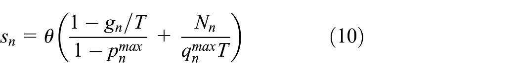
where $θ$ is the adjustment coefficient of number of stops, usually using 0.9.

Effective capacity

The effective capacity during phase n is formulated as

$ca p_{n} = a^{ij} [\frac{(t_{n} - l_{n})}{h^{ij} + 1}]$ (13)

$t_{n} = g_{n} + Y_{n} + R_{n}$ (14)

$g_{n} = {\begin{matrix} g_{n}^{\max}, & g'_{n} > g_{n}^{\max} \\ g_{n}^{\min}, & g'_{n} < g_{n}^{\min} \\ g'_{n}, & otherwise \end{matrix}$ (15)

$g'_{n} = (q_{n}^{\max} - 1) h^{ij} - Y_{n} + l_{n}$ (16)

$q_{n}^{ij} = μ_{n}^{ij} t'_{n} + q_{n, H}^{ij} - a^{ij} [\frac{(t_{n, H} - l_{n, H})}{h^{ij} + 1}]$ (17)

$t'_{n} = t_{n}^{H} + t_{n}^{C} + t_{n}$ (18)

where $h^{ij}$ is the saturated time headway of vehicles from entering leg i to exit leg j; $q_{n}^{ij}$ the actual traffic volume intending to cross the intersection from entering leg i to exit leg j during phase n, consists of three items, as shown in equation (17), the first item $μ_{n}^{ij} t'_{n}$ is the number of arrival vehicles from the end of phase n during last cycle to the end of phase n during current cycle, the second item $q_{n, H}^{ij}$ is the traffic volume corresponding to $q_{n}^{ij}$ during last cycle, and the third item $a^{ij} [(t_{n, H} - l_{n, H}) / h^{ij} + 1]$ is the number of vehicles leaving the intersection during phase n of last cycle; $t_{n, H}$ shows the phase time corresponding to $t_{n}$ during last cycle; $l_{n, H}$ indicates the lost time corresponding to $l_{n}$ during last cycle; $g'_{n}$ is the displayed green time obtained from $q_{n}^{max}$ ; $t_{n}^{H}$ is the time from the end of phase n during last cycle to the end of last cycle; $t_{n}^{C}$ is the time from the beginning of current cycle to the beginning of current phase n.

Therefore, the multi-objective traffic signal control model is generally formulated as the following equation

$\begin{matrix} f_{1} (t_{n}) = min D = \sum_{n = 1}^{N} (d_{n} \cdot q_{n}) / \sum_{n = 1}^{N} q_{n} \\ f_{2} (t_{n}) = min S = \sum_{n = 1}^{N} (s_{n} \cdot q_{n}) / \sum_{n = 1}^{N} q_{n} \\ f_{3} (t_{n}) = max Cap = \sum_{n = 1}^{N} ca p_{n} / N \\ s . t . {\begin{matrix} g_{n}^{\min} \leq g_{n} \leq g_{n}^{\max} \\ g_{n} = g_{en} - Y_{n} + l_{n} \\ t_{n} = g_{n} + Y_{n} + R_{n} \\ \begin{matrix} T = \sum_{n = 1}^{N} t_{n} \\ n = 1, 2, \dots, N \end{matrix} \end{matrix} \end{matrix}$ (19)

In this model, the time-varying turning movement flows are estimated from detected entering and exiting volumes using dynamic origin–destination estimation methods. Furthermore, since the input data are time-varying, this model could obtain real-time signal timing plan for intersections.

PSO algorithm based on Pareto front

PSO algorithm is a very efficient method especially applicable to multi-objective, nonlinear, discontinuous, and non-differentiable optimization problems. Meanwhile, in this article, we have three objectives in the nonlinear traffic signal control model. There exist interactions and contradicts among different objectives, and optimization of one objective usually causes inferiority of other objectives. Pareto front, that is, non-dominated solution set, has been proved to be very applicable to handle this problem. Therefore, we integrate Pareto front into the PSO algorithm for solution of the multi-objective real-time signal control model in equation (19).

Some key issues in the PSO algorithm based on Pareto front are illustrated as follows. Integration process of Pareto front and PSO algorithm is also presented in detail in this section.

Variable definitions

The global best PSO algorithm is employed in this article. There are totally M particles (usually 10–50), and each particle flies in an N-dimensional space at a certain velocity. In the searching process of the best flying path, considering the position change based on its and other particles’ historical best positions in the global search, the particle m has three N-dimensional vector attributes, as follows:

Current position: $t_{m} = (t_{m, 1}, t_{m, 2}, \dots, t_{m, n}, \dots, t_{m, N})$

Historical best position: $p_{m} = (p_{m, 1}, p_{m, 2}, \dots, p_{m, n}, \dots, p_{m, N})$

Velocity: $v_{m} = (v_{m, 1}, v_{m, 2}, \dots, v_{m, n}, \dots, v_{m, N})$

where $m = 1, 2, \dots, M$ ; current position is the signal time of each phase, which is actually a set of coordinate denoting spatial point in the PSO algorithm. In each iteration step of the algorithm, the current position is taken as the solution of multi-objective problem to compute evaluation index, that is, fitness function of the algorithm. Based on the fitness function of the current position, the Pareto dominance relation and density distance among particles are obtained. Furthermore, according to tournament selection strategy, if the fitness value of the current position is better than that of historical best position $p_{m}$ , $p_{m}$ is updated. Meanwhile, if the fitness value of the best particle is better than that of global best position, the global best position, that is, $gbest = (gbes t_{1}, gbes t_{2}, \dots, gbes t_{n}, \dots, gbes t_{N})$ , is updated.

Position and velocity updating mechanism

During the iterative searching process, each particle updates its position and velocity according to historical individual best position and historical global best position. Position and velocity updating mechanisms are illustrated in the following equations

$t_{m, n} (l + 1) = t_{m, n} (l) + v_{m, n} (l + 1)$ (20)

$\begin{matrix} v_{m, n} (l + 1) = ω v_{m, n} (l) + c_{1} \times rand (0, 1) \\ \times [p_{m, n} - t_{m, n} (l)] + c_{2} \times rand (0, 1) \\ \times [gbes t_{n} - t_{m, n} (l)] \end{matrix}$ (21)

where l is the index of iteration; $l_{max}$ is the maximum number of iterations; $ω$ is the inertia weight of PSO algorithm; $rand (0, 1)$ is a random function within the range [0, 1], following a uniform distribution; $c_{1}$ is the relative weight of local search; $c_{2}$ is the relative weight of global search.

In the velocity updating equation (21), the first item reflects the influence of the current velocity, which relates the status of the particle in last iteration and balances the local and global searches; the second item indicates the influence of the cognitive mode, which relates historical memory of the particle and enables the global search ability; the third item shows global information of particle swarm and reflects information sharing and interactions among particles.

Parameters

Inertia weight

Inertia weight could realize effective control and adjustment of particle’s flying velocity. Rather big inertia weight tends to global search, while rather small inertia weight tends to local search. The most simple inertia weight is a fixed value. Dynamic inertia weight is usually utilized to speed up the global search process with a big value in the early period and to improve the local search accuracy with a small value in the late period. Therefore, dynamic inertia weight is used frequently in PSO algorithm, such as linear descending weight, nonlinear weight, adaptive weight, and random weight. Shrinkage factor is also used in place of inertia weight to avoid too small weight in the late period, which will lose the ability of searching new space.

1. Fixed inertia weight

Fixed inertia weight has been proved effective within the range [0.4, 1.4].

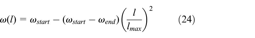
2. Linear descending inertia weight

Formulation 1

$ω (l) = ω_{start} - (ω_{start} - ω_{end}) (\frac{l}{l_{\max}})$ (22)

Formulation 2

$ω (l) = ω_{start} - (ω_{start} - ω_{end}) (\frac{l_{\max} - l}{l_{\max}})$ (23)

where $ω_{start}$ is the initial inertia weight, usually taken as 0.9; $ω_{end}$ is the inertia weight in the last iteration, usually taken as 0.4; l is still the index of iteration. Obviously, inertia weight decreases with the increase in iteration number.

3. Nonlinear inertia weight

Formulation 1

$ω (l) = ω_{start} - (ω_{start} - ω_{end}) {(\frac{l}{l_{\max}})}^{2}$ (24)

Formulation 2

$ω (l) = ω_{start} - (ω_{start} - ω_{end}) [\frac{2 l}{l_{\max}} - {(\frac{l}{l_{\max}})}^{2}]$ (25)

Formulation 3

$ω (l) = ω_{end} {(\frac{ω_{start}}{ω_{end}})}^{1 / (1 + 10 l / l_{\max})}$ (26)

4. Adaptive inertia weight

$ω (l) = ω_{start} - \frac{l (ω_{start} - ω_{end})}{l_{\max}}$ (27)

5. Random inertia weight

${\begin{matrix} ω (l) = μ + σ \cdot N (0, 1) \\ μ = ω_{end} + (ω_{start} - ω_{end}) \cdot rand (0, 1) \end{matrix}$ (28)

where $N (0, 1)$ is a random number following stand normal distribution; $rand (0, 1)$ is a random number following uniform distribution; $σ$ is the variance of random weight, which is usually taken as 0.2.

6. Shrinkage factor

$v_{m, n} (l + 1) = φ {v_{m, n} (l) + c_{1} \times r a n d (0, 1) \times [p_{m, n} - t_{m, n} (l)] + c_{2} \times r a n d (0, 1) \times [g b e s t_{n} - t_{m, n} (l)]}$ (29)

where $φ$ is the shrinkage factor, $φ = (2) / (| 2 - C - \sqrt{C^{2} - 4 C} |)$ ; $C = c_{1} + c_{2}$ , and usually $C > 4$ .

All the above inertia weights are employed in the case study for scenario analyses, and the best inertia weight is then determined.

Acceleration constant

As defined in the above section, $c_{1}$ and $c_{2}$ are the two nonnegative acceleration constants, representing particle’s abilities of self-learning and learning from other excellent particles, respectively. They are employed as fixed values, synchronous change, or asynchronous change during the iteration process, as follows:

1. Fixed values: within the range [0, 4], and the sum of $c_{1}$ and $c_{2}$ is 4.

2. Synchronous change

$c_{1} = c_{2} = \frac{c_{max} - c_{min}}{l_{max}} \cdot l$ (30)

where $c_{max}$ and $c_{min}$ are the maximum and minimum values of acceleration constant, respectively. Usually, $c_{max} = 4$ , $c_{min} = 0$ .

3. Asynchronous change

${\begin{matrix} c_{1} = c_{1, ini} + \frac{c_{1, fin} - c_{1, ini}}{l_{max}} \cdot l \\ c_{2} = c_{2, ini} + \frac{c_{2, fin} - c_{2, ini}}{l_{max}} \cdot l \end{matrix}$ (31)

where $c_{1, ini}$ and $c_{2, ini}$ are the initial values of $c_{1}$ and $c_{2}$ , respectively; $c_{1, fin}$ and $c_{2, fin}$ are the final values of $c_{1}$ and $c_{2}$ , respectively. Usually, $c_{1, ini} = 2.5$ , $c_{2, ini} = 0.5$ , $c_{1, fin} = 0.5$ , and $c_{2, fin} = 2.5$ .

All the above three kinds of acceleration constants are employed in the case study for scenario analyses, and the best $c_{1}$ and $c_{2}$ are then determined.

Maximum particle velocity

$V_{\max}$ is a constant indicating the maximum velocity. It is usually taken as the maximum value at the current position. $V_{\max}$ restricts the velocity within the range $[- V_{\max}, V_{\max}]$ , that is

${\begin{matrix} v_{m, n} = - V_{\max} & if v_{m, n} < - V_{max} \\ v_{m, n} = V_{\max} & if v_{m, n} > V_{max} \end{matrix}$ (32)

Density distance

The Euclidean distance $d_{ij}$ is employed to denote the distance between particles i and j, then the distance matrix of M particles is represented as

$Dist = [\begin{matrix} d_{11} & d_{12} & \dots & d_{1 M} \\ d_{21} & d_{22} & \dots & d_{2 M} \\ ⋮ & ⋮ & ⋮ & ⋮ \\ d_{M 1} & d_{M 2} & \dots & d_{MM} \end{matrix}]$ (33)

Sorting all Euclidean distances between particle m and other individuals in the feasible solution set, and taking $d_{m}^{1}$ and $d_{m}^{2}$ as the shortest two distances, then the density distance of particle m is formulated as

$D d_{m} = \frac{(d_{m}^{1} + d_{m}^{2})}{2}$ (34)

In the same grade of Pareto dominance relation, with the increase in density distance, the particles change to be non-congested, and the diversity of the particles turns to be more obvious. Besides the above parameters, the size of particle swarm and number of iterations are also very important for PSO algorithm. Different values of them are also designed for scenario analyses in the case study, and the best values are then decided. All the above parameters maintain the balance between global and local search abilities and ensure the implementation of PSO algorithm process.

Algorithm flow

Based on the above explanations, a step-by-step flow is designed for the Pareto front–based PSO algorithm. The graphical illustration is shown in Figure 2.

Figure 2.

Flow chart of PSO algorithm based on Pareto front.

The flow is further described in detail as follows:

Step 1: let iteration index l equal to 0, and initialize the parameters of PSO algorithm, including historical best position of particle, global best position, position and velocity of particle, and some other parameters.

Step 2: compute fitness value of the particle according to fitness function, calculate density distance of each particle, and sort particles in the same grade of Pareto dominance relation according to density distance.

Step 3: search local best position of the particle and global best position of particle swarm using tournament selection principle according to ranking based on Pareto dominance relation and density distance.

Step 4: let $l = l + 1$ , update the inertia weight, and then update position and velocity of particle according to equations (20) and (21).

Step 5: update fitness value of the particle, calculate density distance of each particle, and sort particles in the same grade of Pareto dominance relation again according to density distance.

Step 6: update local best position of particle and global best position of particle swarm using tournament selection principle again.

Step 7: repeat Steps 4–6 until preset iteration number or accuracy requirement is arrived, and let each particle fall within Pareto front.

Step 8: terminate the algorithm, and output optimal real-time traffic signal timing plan as well as evaluation indices.

The above Pareto front–based PSO algorithm is coded using M language based on MATLAB platform.

Case study

To testify performances of the proposed multi-objective traffic control model and Pareto front–based PSO algorithm, we implemented a survey on a Wednesday morning at the intersection of Zhao Dengyu Road and Pinganli West Street in Beijing, China. We collected real-time link traffic volume and turning movement flow of totally 3 h, including both peak and nonpeak hours. We also gathered geometric features of the intersection, the current signal timing parameters, delay time, saturated time headway, and other necessary information. All the above data provided rather rich input and evaluation indices for the case study. Additionally, we preset the following constants in the signal timing plan: yellow time of each phase, 3 s; all red time of each phase, 1 s; minimum displayed green time, 15 s; maximum displayed green time, 45 s.

We implemented the proposed model and algorithm using MATLAB platform. Here, the case study mainly consists of four parts: scenario analyses of PSO parameters, comparison between the proposed model and current signal timing plan, comparison between the proposed model and traditional method (a pseudo multi-objective traffic control model), and influence of emergency.

Scenario analyses of PSO parameters

To determine the important parameters in the PSO algorithm, we first design some scenarios for the experiments. Here, inertia weight, acceleration constant, particle swarm size, and iteration number are taken for scenario analyses.

Inertia weight

As stated before, there are many kinds of inertia weights. For comparison, we first design some scenarios for fixed inertia weight, and the corresponding evaluation indices of the proposed model are summarized in Table 1.

Table 1.

Comparisons among fixed inertia weights.

Fixed inertia weight	Delay time (s)	Number of stops	Effective capacity (pcu)
0.1	24.9	0.3743	49
0.2	23.2	0.3353	49
0.3	23.3	0.3424	49
0.4	23.1	0.3373	51
0.5	24.6	0.3727	49
0.6	24.0	0.3488	50
0.7	26.7	0.4012	49
0.8	24.1	0.3471	50
0.9	24.6	0.3507	50
1.0	24.4	0.3470	51
1.1	26.3	0.3935	53
1.2	25.1	0.3885	52
1.3	20.7	0.3183	48
1.4	21.0	0.3396	48

The italic values show that the model effect is the best while the fixed inertia weight equals to 0.4.

From Table 1, we can find out that model effect is the best while the fixed inertia weight equals to 0.4. Therefore, 0.4 is employed as the representative of fixed inertia weight in the following analyses.

We further utilize linear descending weight (including Formulations 1 and 2), nonlinear weight (including Formulations 1, 2, and 3), adaptive weight, random weight, and shrinkage factor in the scenario analysis, and the comparisons of the three indices are shown in Table 2.

Table 2.

Scenario analysis of inertia weight.

Fixed inertia weight	Delay time (s)	Number of stops	Effective capacity (pcu)
Fixed	23.1	0.3373	51
Linear: 1	24.5	0.3545	51
Linear: 2	22.9	0.3313	49
Nonlinear: 1	25.1	0.3703	50
Nonlinear: 2	26.0	0.3760	51
Nonlinear: 3	26.3	0.3858	50
Adaptive	24.6	0.3551	52
Random	20.0	0.2983	50
Shrinkage factor	22.8	0.3339	49

The italic values indicate that random inertia weight is the best in all alternatives.

Graphical illustrations are further presented in Figures 3 –5.

Figure 3.

Delay time at different inertia weights.

Figure 4.

Number of stops at different inertia weights.

Figure 5.

Effective capacity at different inertia weights.

From the above tables and figures, we can find out that random inertia weight is generally the best in all alternatives. Therefore, we employ random inertia weight in the following analyses.

Acceleration constant

As stated in the previous section, we design scenarios in Table 3 for acceleration constant.

Table 3.

Scenarios of acceleration constant.

Acceleration constant	Scenarios
c ₁	0	1	1	1	1.5	1.5	2	2	2	2.5	4	S-c	As-c
c ₂	2	1	1.5	2	1	1.5	0	1	2	1.5	0	S-c	As-c

S-c: synchronous change; As-c: asynchronous change.

Graphical illustrations of evaluation indices at different acceleration constants are reported in Figures 6 –8.

Figure 6.

Delay time at different acceleration constants.

Figure 7.

Number of stops at different acceleration constants.

Figure 8.

Effective capacity at different acceleration constants.

From the above three figures, we can find out that the fixed acceleration constant pair 2–2 is the best choice. Therefore, we employ the fixed acceleration constant (2–2) in the following analyses.

Particle swarm size

Particle swarm size influences accuracy and efficiency greatly. Since the size usually falls within the range from 10 to 50, we set it as 10, 20, 30, 40, and 50, respectively, for scenario analysis. Table 4 summarizes the average CPU time for each signal cycle, which is output using MATLAB software.

Table 4.

Average CPU time for each signal cycle at different particle swarm sizes.

Particle swarm size	10	20	30	40	50
Average CPU time (s)	0.7	2.4	5.4	9.4	15.2

Three evaluation indices at different particle swarm sizes are further illustrated in Figures 9 –11.

Figure 9.

Delay time at different particle swarm sizes.

Figure 10.

Number of stops at different particle swarm sizes.

Figure 11.

Effective capacity at different particle swarm sizes.

Considering optimization effects and calculation efficiency together, we finally select 20 as the particle swarm size in the following analyses.

Iteration number

Big iteration number usually improves the accuracy of PSO algorithm; however, it will also greatly influence the efficiency. Based on random inertia weight, fixed acceleration, and particle swarm of 20, we further set iteration number as 20, 50, 100, and 200, respectively, for scenario analysis. Table 5 reports the average CPU time for each signal cycle

Table 5.

Average CPU time for each signal cycle at different iteration numbers.

Particle swarm size	20	50	100	200
Average CPU time (s)	0.7	37.9	80.9	1957.7

Three evaluation indices at different iteration numbers are further presented in Figures 12 –14.

Figure 12.

Delay time at different iteration numbers.

Figure 13.

Number of stops at different iteration numbers.

Figure 14.

Effective capacity at different iteration numbers.

Overall consideration of optimization effects and calculation efficiency obviously shows that 20 is the best choice for iteration number.

Based on the above scenario analyses, we finally set PSO parameters as follows and apply them in the consequent analyses:

Inertia weight: random inertia weight;

Acceleration constant: relative weights of local and global searches are both 2;

Particle swarm size: 20;

Iteration number: 20.

Comparison between the proposed model and current scheme

To testify the effects of the proposed model, we further compare the signal timing plan from it with the current signal scheme. The results show that totally 74 cycles are obtained, as shown in Figure 15.

Figure 15.

Real-time cycle length of the proposed model.

Different from current fixed timing, signal cycle from the proposed model is real-time, that is, it is applicable to time-varying travel demand. Furthermore, the average cycle length is 146 s during all 3 h from 7:00 a.m. to 10:00 a.m., 150 s during peak hours from 7:00 a.m. to 8:30 a.m., and 142 s during nonpeak hours from 8:30 a.m. to 10:00 a.m. Obviously, the average cycle length during peak hours is longer than that during nonpeak hours, and the cycle adjusts dynamically along with time-varying traffic flows.

We surveyed the average delay time for control effect comparison. Moreover, we calculated the capacity of the intersection under the existing signal timing. These two indices are employed for comparisons. The average delay time and effective capacity of the proposed model and current signal scheme are compared in Figures 16 and 17, respectively.

Figure 16.

Delay time comparison between proposed model and current scheme.

Figure 17.

Effective capacity comparison between proposed model and current scheme.

It is obvious that delay time at each entrance leg from the proposed model is less than that of the current scheme, as well as the average delay time. Meanwhile, effective capacity at each entering approach from the proposed model is greater than that of the current scheme except for the east entrance, and the average capacity of the proposed model is much larger than that of the current scheme. Therefore, the real-time signal timing plan from the proposed model is much more effective than the current signal scheme and is applicable to dynamic traffic flows.

Comparison between the proposed model and pseudo multi-objective method

As stated before, the existing multi-objective traffic control model usually converts into single-objective problem using weighted sum method, that is, pseudo multi-objective model. To testify the applicability of Pareto front in the proposed model, we also formulate a pseudo multi-objective model using the proposed objectives for comparison.

The objective of the pseudo method is

$f (t_{n}) = min \sum_{n = 1}^{N} [K_{n}^{1} d_{n} + K_{n}^{2} s_{n} - K_{n}^{3} ca p_{n}]$ (35)

where $K_{n}^{1}$ , $K_{n}^{2}$ , and $K_{n}^{3}$ are the three weight coefficients for single-objective conversion; $K_{n}^{1} = q_{n} (1 - P)$ ; $K_{n}^{2} = q_{n} (1 - P) T$ ; $K_{n}^{3} = P$ ; P is the volume-to-capacity ratio during the cycle.

Using the above three weights, the objective lays particular emphasis on delay time and number of stops during nonpeak hours, while on effective capacity during peak hours. Equations (1)–(4) and (35) constitute the pseudo multi-objective control model together.

Comparisons of some signal parameters are summarized in Table 6.

Table 6.

Signal timing plans from different models.

Model	Number of cycles	Average cycle length (s)	Peak average cycle length (s)	Nonpeak average cycle length (s)
Current scheme	68	159	159	159
Proposed model	74	146	150	142
Pseudo model	124	87	92	83

Obviously, the number of cycles from the pseudo model increases dramatically, together with the sharp decrease in the average cycle length. Three evaluation indices are further illustrated in Figures 18 –20.

Figure 18.

Delay time comparison between proposed model and pseudo multi-objective model.

Figure 19.

Number of stops’ comparison between proposed model and pseudo multi-objective model.

Figure 20.

Effective capacity comparison between proposed model and pseudo multi-objective model.

We can find out that delay time at each entering leg from the pseudo multi-objective model is much larger than that of the proposed methodology, as well as the number of stops. Meanwhile, effective capacity at each entering leg from the pseudo model is much smaller than that of the proposed model. All these results indicate that the proposed methodology outperforms the pseudo multi-objective model greatly. The possible reason is that the single objective of the pseudo model is the weighted sum of three objectives during one signal cycle, and total delay time and number of stops will increase quickly with the extension of cycle length, which causes rather small value of cycle. Short signal cycle further induces frequent phase change and big time loss, resulting in unsatisfying effects. The above comparisons also prove advantages of Pareto front approach in multi-objective optimization model.

Influence of emergency

Most input data of signal control system are from traffic detection facilities. Sometime emergencies will happen with detectors, for instance, there are some outliers in the detected traffic volume, or some detectors are damaged and fail to input new data suddenly. To testify the robustness of the proposed methodology under such emergencies, we further design this experiment.

Two scenarios are designed for robustness tests:

There are some outliers in the detected traffic volume at east entrance, within a range of ±100%, that is, from 0 to double.

Detectors at east entrance fail thoroughly, that is, there is detected input data at east entering approach, and we duplicate detections at west entrance for east approach temporarily.

We also implement the above two scenarios using MATLAB code. Signal timing plans are summarized in Table 7.

Table 7.

Average signal timing plans under emergencies.

Scenario	Number of cycles	Average cycle length (s)	Average phase time for go straight at east-west direction (s)
Normal	74	146	36
Scenario 1: input outliers	73	148	36
Scenario 2: total failure	81	133	25

It is obvious that under Scenario 1, the signal timing plan remains almost unchanged, that is, the proposed model and algorithm work well in the presence of input outliers, even during peak hours. Comparatively, total failure of the detectors influences signal timing more greatly, because traffic volume at east entering approach is much bigger than that at west entrance, as well as the delay time and queue length, and substitution of detections at west approach increases the number of cycles. However, the intersection is still under regular operation, and the delay time does not increase too much, which can be found out from the following analyses.

Three evaluation indices are further illustrated in Table 8.

Table 8.

Evaluation indices under emergencies.

Scenario	Delay time (s)	Number of stops	Effective capacity (pcu)
Normal	20.0	0.2983	50
Scenario 1: input outliers	20.8	0.3005	52
Scenario 2: total failure	20.3	0.3129	42

From Table 8, we can further find out that all three evaluation indices fall within very narrow ranges under emergencies. Even under total failure of some detectors, delay time still remains almost unchanged. Therefore, the proposed Pareto front–based multi-objective traffic signal control model using PSO algorithm is robust enough for on-line applications in real-time traffic control systems.

Generally, we reach the following results from the above case studies:

Comprehensively considering accuracy and efficiency, scenario analyses provide the most appropriate PSO parameters for the proposed multi-objective traffic control model, including random inertia weight, fixed acceleration constants (c₁ = c₂ = 2), particle swarm size 20, and iteration number 20.

Comparison between the proposed model and current scheme indicates that the multi-objective traffic control model provides real-time signal timing plan applicable to time-varying traffic flow and obtains better delay time, number of stops, and effective capacity than the current signal scheme.

Comparison with the traditional method shows that the proposed methodology outperforms the existing pseudo multi-objective traffic control model, which converts several objectives into single target using weighted sum method. It also proves the advantages of Pareto front in multi-objective optimization problems.

Under emergencies such as input outliers and total failure of detectors, the proposed methodology still works well, which demonstrates its robustness in on-line traffic control systems.

Conclusion

This article presents a general methodology for real-time traffic control at intersections, including a multi-objective optimization model and the corresponding Pareto front–based PSO algorithm. We first formulate a traffic control model for intersections based on detected time-varying traffic flows with three independent objectives, including minimum average delay time, minimum average number of stops, and maximum effective capacity. Second, according to both nonlinear and multi-objective characteristics of the proposed model, we design a PSO algorithm based on Pareto front for solution. The proposed methodology provides real-time traffic signal timing plan for intersections, including time-varying cycle and split. Using actual survey data, we further implement case studies to testify performances of the methodology, including scenario analyses of PSO parameters, comparison between the proposed model and current situation, comparison between the proposed model and traditional method, and influence of emergency. Scenario analyses give the most appropriate PSO parameters, comparison with the current situation indicates effectiveness of the proposed method, comparison with traditional approach proves the applicability of Pareto front in multi-objective problem, and influence of emergency demonstrates robustness of the proposed methodology. Generally, the Pareto front–based multi-objective real-time traffic signal control model for intersections using PSO algorithm is effective and robust enough for on-line applications.

This article can be developed toward following directions. The first is to comprehensively consider upstream and downstream junctions to formulate multi-objective traffic control models for urban arterial roads. The second is to develop multi-objective models for urban regional coordination control. The third is to design other swarm intelligence algorithms for solution and to compare them with Pareto front–based PSO algorithm.

Footnotes

Valuable comments and suggestions from anonymous reviewers are gratefully acknowledged.

Academic Editor: Gang Chen

Declaration of conflicting interests

The author(s) declared no potential conflicts of interest with respect to the research,authorship,and/or publication of this article.

Funding

The author(s) disclosed receipt of the following financial support for the research,authorship,and/or publication of this article: This research was supported by National Natural Science Foundation of China (51578040),Beijing Nova Programme of China (Z151100000315050),Beijing Natural Science Foundation Project (8162013),Distinguished Young Scholars Program of Beijing University of Civil Engineering and Architecture,and Importation and Development of High-Caliber Talents Project of Beijing Municipal Institutions (CIT&TCD201404071).

References

Gazis

DC.

Optimum control of a system of oversaturated intersections. Oper Res 1964; 12: 815–831.

D’Ans

Gazis

DC.

Optimal control of oversaturated store-and-forward transportation networks. Transport Sci 1976; 10: 1–19.

Jiao

Liu

. Real-time traffic signal optimization model based on average delay time per person. Adv Mech Eng. Epub ahead of print 29 October 2015. DOI: 10.1177/1687814015613500.

Michalopoulos

Stephanopoulos

Oversaturated signal systems with queue length constraints—I: single intersection. Transport Res 1977; 11: 413–421.

Michalopoulos

Stephanopoulos

Oversaturated signal systems with queue length constraints—II: systems of intersections. Transport Res 1977; 11: 423–428.

Michalopoulos

Stephanopoulos

Optimal control of oversaturated intersections: theoretical and practical considerations. Traffic Eng Contr 1978; 19: 216–221.

Ahn

Machemehl

RB.

Methodology for traffic signal timing in oversaturated arterial networks (research report SWUTC/98/465510-1). Alexandria, VA: National Technical Information Service, 1997.

Lieberman

Chang

Prassas

ES.

Formulation of real-time control policy for oversaturated arterials. Transp Res Rec 2000; 1727: 77–88.

Ceder

Reshetnik

An algorithm to minimize queues at signalized intersections. J Oper Res Soc 2001; 52: 615–622.

10.

Talmor

Mahalel

Signal design for an isolated intersection during congestion. J Oper Res Soc 2007; 58: 454–466.

11.

Jiao

Sun

Multiobjective traffic signal control model for intersection based on dynamic turning movements estimation. Math Probl Eng 2014; 2014: 608194 (8 pp.).

12.

Schmöcker

J-D

Ahuja

Bell

MGH

. Multi-objective signal control of urban junctions—framework and a London case study. Transport Res C: Emer 2008; 16: 454–470.

13.

Shou

. Multi-objective optimization of oversaturated signalized intersection based on fuzzy logic. In: Proceedings of the 8th World Congress on Intelligent Control and Automation, vol. 20, no. 1, Jinan, China, 7–9 July 2010, pp.5008–5013. New York: IEEE.

14.

Robertson

DI.

TRANSYT: a traffic network study tool (RRL report LR 253). UK: Road Research Laboratory, 1969.

15.

Wallace

Courage

Reaves

. TRANSYT-7F user’s manual (technical report UF-TRC-U32 FP-06/07). Gainesville, FL: University of Florida, 1988.

16.

Wong

SC.

Group-based optimisation of signal timings using the TRANSYT traffic model. Transport Res B: Meth 1996; 30: 217–244.

17.

Sim

AG.

The Sydney coordinated adaptive traffic (SCAT) system philosophy and benefits. IEEE T Veh Technol 1980; 29: 130–137.

18.

Lowrie

. The Sydney coordinated adaptive control system—principles, methodology, algorithms. In: Proceedings of the IEE conference publication, 1982, https://trid.trb.org/view.aspx?id=1188851

19.

Gartner

OPAC: a demand-responsive strategy for traffic signal control. Transp Res Rec 1983; 906: 75–81.

20.

Bretherton

Bowen

GT.

Recent enhancements to SCOOT—SCOOT version 2.4. In: Proceedings of the 3rd international conference on road traffic control, London, 1–3 May 1990, pp.95–98. New York: IEEE.

21.

Robertson

Bretherton

RD.

Optimizing networks of traffic signals in real-time: the SCOOT method. IEEE T Veh Technol 1991; 40: 11–15.

22.

Mirchandani

Head

A real-time traffic signal control system: architecture, algorithms, and analysis. Transport Res C: Emer 2001; 9: 415–432.

23.

Jiao

Yang

. Real-time estimation of turning movement proportions based on genetic algorithm. In: Proceedings of the 8th international IEEE conference on intelligent transportation systems, Vienna, 13–15 September 2005, pp.484–489. New York: IEEE.

24.

Jiao

Sun

A Bayesian combined model for time-dependent turning movement proportions estimation at intersections. Math Probl Eng 2014; 2014: 607195 (8 pp.).

25.

Jiao

Wang

Sun

Real-time arterial coordination control based on dynamic intersection turning fractions estimation using genetic algorithm. Math Probl Eng 2014; 2014: 430497 (10 pp.)

26.

Jiao

Liu

Guo

. Bi-bayesian combined model for two-step prediction of dynamic turning movement proportions at intersections. Adv Mech Eng 2014; 2014: 439031 (9 pp.).

27.

Song

Guan

. k-Nearest neighbor model for multiple-time-step prediction of short-term traffic condition. J Transp Eng: ASCE 2015; 142, http://ascelibrary.org/doi/abs/10.1061/(ASCE)TE.1943-5436.0000816

28.

Yao

Zhang

. Improved support vector machine regression in multi-step-ahead prediction for rock displacement surrounding a tunnel. Sci Iran 2014; 21: 1309–1316.

29.

Yao

Zhang

. A support vector machine with the tabu search algorithm for freeway incident detection. Int J Appl Math Comp 2014; 24: 397–404.

30.

Kennedy

Eberhart

Particle swarm optimization. In: Proceedings of the IEEE international conference on neural networks, Piscataway, NJ, 27 November–1 December 1995, pp.1942–1948. New York: IEEE.

31.

Eberhart

Kennedy

A new optimizer using particle swarm theory. In: Proceedings of the 6th international symposium on micro machine and human science, Nagoya, Japan, 4–6 October 1995, pp.39–43. New York: IEEE.

32.

Bashir

El-Hawary

. Short-term load forecasting using artificial neural network based on particle swarm optimization algorithm. In: Proceedings of the Canadian conference on electrical and computer engineering, Vancouver, BC, Canada, 22–26 April 2007, pp.272–275. New York: IEEE.

33.

Mendes

Kennedy

Neves

The fully informed particle swarm: simpler, maybe better. IEEE T Evolut Comput 2004; 8: 204–210.

34.

Espitia

Sofrony

. Path planning of mobile robots using potential fields and swarms of Brownian particles. In: Proceedings of the 2011 IEEE Congress of Evolutionary Computation, New Orleans, LA, 5–8 June 2011, pp.123–129. New York: IEEE.

35.

Ding

Zhou

Phase angle-encoded and quantum-behaved particle swarm optimization applied to three-dimensional route planning for UAV. IEEE T Syst Man Cy A 2012; 42: 511–526.

36.

Yao

. Transit network design based on travel time reliability. Transport Res C: Emer 2014; 43: 233–248.

37.

Kong

Sun

. A bi-level programming for bus lane network design. Transport Res C: Emer 2015; 55: 310–327.

38.

Mostaghim

Teich

. Strategies for finding good local guides in multi-objective particle swarm optimization (MOPSO). In: Proceedings of the 2003 IEEE swarm intelligence symposium, Indianapolis, IN, 24–26 April 2003, pp.26–33. New York: IEEE.

39.

Tripathi

Bandyopadhyay

Pal

SK.

Multi-objective particle swarm optimization with time variant inertia and acceleration coefficients. Inform Sciences 2007; 177: 5033–5049.

40.

Reyes-Sierra

Coello Coello

CA.

Multi-objective particle swarm optimizers: a survey of the state-of-the-art. Int J Comput Intell Res 2006; 2: 287–308.

41.

Yao

. An improved particle swarm optimization for carton heterogeneous vehicle routing problem with a collection depot. Ann Oper Res 2016; 242: 303–320.

42.

Deb

Multiobjective optimization using evolutionary algorithms. New York: John Wiley& Sons, 2001.

43.

Cui

Tao

Genetic algorithm for pareto optimum-based route selection. J Syst Eng Electron 2007; 18: 360–368.

44.

Meng

Khoo

HL.

A Pareto-optimization approach for a fair ramp metering. Transport Res C: Emer 2010; 18: 489–506.

45.

Stevanovic

Kergaye

Optimization of traffic signal timings based on surrogate measures of safety. Transport Res C: Emer 2013; 32: 159–178.

46.

El-Alfy

ESM

Mujahid

Selim

SZ.

A Pareto-based hybrid multiobjective evolutionary approach for constrained multipath traffic engineering optimization in MPLS/GMPLS networks. J Netw Comput Appl 2013; 36: 1196–1207.

47.

Akcelik

Time-dependent expressions for delay, stop rate and queue length at traffic signals (internal report AIR 367-1). Vermont South, VIC, Australia: Australian Road Research Board, 1980.

Pareto front–based multi-objective real-time traffic signal control model for intersections using particle swarm optimization algorithm

Abstract

Keywords

Introduction

Problem statement and symbol definitions

Multi-objective traffic signal control model

Average delay time

Average number of stops

Effective capacity

PSO algorithm based on Pareto front

Variable definitions

Position and velocity updating mechanism

Parameters

Inertia weight

Acceleration constant

Maximum particle velocity

Density distance

Algorithm flow

Case study

Scenario analyses of PSO parameters

Inertia weight

Acceleration constant

Particle swarm size

Iteration number

Comparison between the proposed model and current scheme

Comparison between the proposed model and pseudo multi-objective method

Influence of emergency

Conclusion

Footnotes

Declaration of conflicting interests

Funding

References