Sage Journals: Discover world-class research

Abstract

Sounding rockets are the only direct detection method for near-space and are utilized for different kinds of scientific research. Dynamic models are the foundation of research on sounding rockets. However, no dynamic models have included all the working processes of a sounding rocket. A high-precision dynamic model of a sounding rocket is proposed in this article; the model includes motion on the launch rail, the free flight phase, parachute deployment, the inflation process, and steady descent. Through the model, the entirety of the dynamic process can be understood in detail to help improve performance. A combination wind compensation method was investigated to rapidly and accurately obtain launch parameters; the method was derived from a wind weighting and pattern search method. Based on the simulation results, the proposed approaches are proven to be effective.

Keywords

Sounding rocket flight dynamics separation dynamics multi-body dynamics wind compensation

Introduction

Sounding rockets, which lack control systems, are simple structures, and their costs are relatively low. The altitude of the trajectory can be changed easily according to the launch mission.^1,2 Sounding rockets can explore the circumstances of near-space and can also be used to perform scientific research in that special environment.^3,4 As a consequence of being the only direct detection method for near-space from tens to hundreds of kilometers, sounding rockets are now widely used in near-space circumstance detection,^5,6 microgravity experiments,⁷ and the validation of new space technologies.⁸

The NASA (National Aeronautics and Space Administration) Sounding Rockets Program has launched more than 40 sounding rockets for different purposes over the past 3 years, including geospace science, astrophysics, solar physics, and the improvement and validation of technologies. Through the work of the sounding rockets, great discoveries in galaxy formation have been found by the team of Dr Bock and Colleagues⁹ and substructures in the solar corona and their impact on coronal heating by the team of Dr Cirtain and Colleagues.¹⁰ These achievements reconfirm that a few minutes of suborbital flight by a sounding rocket can enable world-class scientific discoveries. The total number of launches by NASA in the last 10 years is 184. NASA now has 14 kinds of sounding rocket vehicles, and the apogee altitudes of the rockets range from 50 to more than 1600 km.¹¹

The European Space Agency has been using sounding rockets to conduct low-gravity experiments since 1982. There are now four kinds of sounding rockets that are offered for microgravity research: MiniTexus, Texus, Maser, and Maxus.¹² The German MiniTexus sounding rocket program utilizes a two-stage solid propellant vehicle, the apogee is 140 km, and approximately 3 min of microgravity can be provided. The German Texus program now uses the VSB-30 sounding rocket, which was developed by Germany and Brazil, and through some launch missions from Texus-42 to Texus-48, it can now provide up to 6 min of microgravity. The apogee is 260 km.^13,14 The Maser sounding rocket program was initiated by Sweden, the rocket has similar characteristics to the Texus, with microgravity durations up to 6 min, and the apogee is 260 km. The Maxus sounding rocket program was initiated by an industrial joint venture formed by EADS-ST and the Swedish Space Corporation. The Maxus program offers 12–13 min of microgravity, and the apogee of the trajectory is 705 km.

There are now various software packages we can access to simulate the trajectories of rockets, including RockSim and OpenRocket, which only simulate rockets under nominal conditions, and the Cambridge Rocketry Simulator, which can fly rockets under a range of possible flight conditions to obtain confidence bounds on expected flight paths and landing locations.¹⁵ However, there are no dynamic models that include all of the working processes of sounding rockets. In this article, we will introduce a high-precision dynamic model of a sounding rocket, which consists of motion on the launch rail, free flight, the drawing out and inflation of parachutes, and the steady descent of the sonde–parachute system. In addition, based on the dynamic model, a new method for compensating wind effects is discussed. Based on the work reported in this article, we can determine details of the entire flight process, complete missions more successfully, and safely recover payloads.

The rocket trajectory

Dynamics of the motion on the launch rail

Once the motor is ignited, a rocket moves on the launch rail. When the front directional button has exited the launch rail, the rocket rotates around the aft directional button. A rotational angle and rotational angular velocity, which are commonly called the sinking angle and sinking angle velocity, are therefore produced.

The length of the launch rail is $L$ , the distance between the front directional button and the top of the launch rail is $L_{1}$ , and the distance between the aft directional button and the top of the launch rail is $L_{2}$ , as shown in the reference frame $o - xyz$ in Figure 1.

Figure 1.

The motion on the launch rail.

Linear motion

When the rocket is moving in a straight line in the launch rail direction, the rocket is affected by gravity, thrust, and the friction forces between the rocket and the rail, and the equations of motion can be obtained by Newton’s equation of motion, as shown in equation (1)

${\begin{matrix} {\overset{\cdot}{V}}_{x} = \frac{P - μ G \cos θ_{0} - G \sin θ_{0}}{m} \\ \overset{\cdot}{x} = V_{x} \end{matrix}$ (1)

In equation (1), $V_{x}$ is the component velocity along the axis $ox$ , $P$ is the rocket engine thrust, $G$ is the gravity of the rocket, $θ_{0}$ is the elevation angle of the launch rail, $μ$ is the friction coefficient between the directional button and the launch rail, $m$ is the mass of the rocket, and $x$ is the distance the rocket moves along $ox$ .

Rigid body plane motion

When the rocket is moving in a plane, the forward directional button moves past the launch rail, and gravity produces a torque causing the rocket to begin to rotate around the aft directional button. In addition, the thrust is not in the same direction as the launch rail, as affected by the torque, and the elevation angle of the rocket is now $θ$ . Based on the previous analysis, the equation of motion is shown in equation (2)

${\begin{matrix} {\overset{\cdot}{V}}_{x} = \frac{(P \cos (θ_{0} - θ) - μ [G \cos θ_{0} + P \sin (θ_{0} - θ)] - G \sin θ_{0})}{m} \\ {\overset{\cdot}{V}}_{y} = 0 \\ \overset{\cdot}{x} = V_{x} \\ \overset{\cdot}{y} = V_{y} \\ \overset{\cdot}{ω} = \frac{R [m {\overset{\cdot}{V}}_{x} \cos (θ_{0} - θ) + G \sin θ - P] - L_{c} [G \cos θ + m {\overset{\cdot}{V}}_{x} \sin (θ_{0} - θ)]}{J_{p}} \\ \overset{\cdot}{θ} = ω \end{matrix}$ (2)

In equation (2), $θ$ is the elevation angle of the rocket, $V_{y}$ is the component velocity along axis $oy$ , $y$ is the distance the rocket moves along $oy$ , $ω$ is the rotational velocity, $R$ is the distance along $oy$ between the aft directional button and the axis of symmetry, $L_{c}$ is the distance along $ox$ between the aft directional button and the center of mass of the rocket, and $J_{p}$ is the moment of inertia of the rocket about the aft directional button.

The free flight phase

Once the rocket has taken off from the launch rail, the rocket flies freely in air under the actions of thrust, gravity, and aerodynamic forces. The 6-DoF (six-degree-of-freedom) dynamic equations of the rocket are built using the quaternion method in a body-fixed coordinate system rotating about a series of axes in the order $ψ - φ - γ$ .

A quaternion is a special set composed of four mutually dependent scalar parameters $q_{0}$ , $q_{1}$ , $q_{2}$ , and $q_{3}$ . In this article, the elements of the quaternion are determined by the equations below

${\begin{matrix} q_{0} = \cos \frac{ψ}{2} \cos \frac{θ}{2} \cos \frac{γ}{2} - \sin \frac{ψ}{2} \sin \frac{θ}{2} \sin \frac{γ}{2} \\ q_{1} = - \cos \frac{ψ}{2} \cos \frac{θ}{2} \sin \frac{γ}{2} - \sin \frac{ψ}{2} \sin \frac{θ}{2} \cos \frac{γ}{2} \\ q_{2} = - \cos \frac{ψ}{2} \sin \frac{θ}{2} \sin \frac{γ}{2} - \sin \frac{ψ}{2} \cos \frac{θ}{2} \cos \frac{γ}{2} \\ q_{3} = - \cos \frac{ψ}{2} \sin \frac{θ}{2} \cos \frac{γ}{2} + \sin \frac{ψ}{2} \cos \frac{θ}{2} \sin \frac{γ}{2} \end{matrix}$ (3)

Combine the equations of the centroid dynamics, dynamics moment equations of the centroid, centroid kinematics equations, and the kinematic equations around the centroid. Substituting the quaternions for the Euler angles, we can obtain the 6-DoF model of the rocket presented below

${\begin{matrix} \frac{dm}{dt} = - m_{c} \\ \frac{dX}{dt} = V_{x} (q_{0}^{2} + q_{1}^{2} - q_{2}^{2} - q_{3}^{2}) + 2 V_{y} (q_{1} q_{2} - q_{0} q_{3}) \\ + 2 V_{z} (q_{0} q_{2} + q_{1} q_{3}) \\ \frac{dY}{dt} = 2 V_{x} (q_{1} q_{2} + q_{0} q_{3}) + V (q_{0}^{2} - q_{1}^{2} + q_{2}^{2} - q_{3}^{2}) \\ + 2 V_{z} (q_{2} q_{3} - q_{0} q_{1}) \\ \frac{dZ}{dt} = 2 V_{x} (q_{1} q_{3} - q_{0} q_{2}) + 2 V_{y} (q_{2} q_{3} + q_{0} q_{1}) \\ + V_{z} (q_{0}^{2} - q_{1}^{2} + q_{2}^{2} - q_{3}^{2}) \end{matrix}$ (4)

${\begin{cases} \frac{d V_{x}}{d t} = \frac{ω_{z} V_{y} - ω_{y} V_{z} + (P - F_{x} \cos α \cos β + F_{y} \sin α - F_{z} \cos α \sin β - 2 m g (q_{1} q_{2} + q_{0} q_{3}))}{m} \\ \frac{d V_{y}}{d t} = \frac{ω_{x} V_{z} - ω_{z} V_{x} + (F_{x} \sin α \cos β + F_{y} \cos α + F_{z} \sin α \sin β - m g (q_{0}^{2} - q_{1}^{2} + q_{2}^{2} - q_{3}^{2}))}{m} \\ \frac{d V_{z}}{d t} = \frac{ω_{y} V_{x} - ω_{x} V_{y} + (- F_{x} \sin α + F_{z} \cos β - 2 m g (q_{2} q_{3} - q_{0} q_{1}))}{m} \end{cases}$ (5)

${\begin{matrix} M_{x} = J_{x} \frac{d ω_{x}}{dt} + (J_{z} - J_{y}) ω_{y} ω_{z} \\ M_{y} = J_{y} \frac{d ω_{y}}{dt} + (J_{x} - J_{z}) ω_{x} ω_{z} \\ M_{z} = J_{z} \frac{d ω_{z}}{dt} + (J_{y} - J_{x}) ω_{x} ω_{y} \end{matrix}$ (6)

$[\begin{matrix} {\overset{\cdot}{q}}_{0} \\ {\overset{\cdot}{q}}_{1} \\ {\overset{\cdot}{q}}_{2} \\ {\overset{\cdot}{q}}_{3} \end{matrix}] = \frac{1}{2} [\begin{matrix} - q_{1} & - q_{2} & - q_{3} \\ q_{0} & - q_{3} & q_{2} \\ q_{3} & q_{0} & - q_{1} \\ - q_{2} & q_{1} & q_{0} \end{matrix}] [\begin{matrix} ω_{x} \\ ω_{y} \\ ω_{z} \end{matrix}]$ (7)

In addition, the geometry equation is given by equation (8)

${\begin{matrix} tg α = \frac{V_{y}}{V_{x}} \\ tg β = \frac{V_{z}}{\sqrt{V_{x}^{2} + V_{y}^{2}}} \end{matrix}$ (8)

In the equations above, $m$ is the mass of the rocket, $V_{i}$ is the velocity along the axes $i$ in the body-fixed coordinates, $M_{i}$ is the moment along the axes $i$ in the body-fixed coordinates, $q_{i}$ is the quaternion ( $i = 0, 1, 2, 3$ ), and $J_{i}$ is the moment of inertia along the axes $i$ in the body-fixed coordinates. $X, Y, and Z$ are the position coordinates in a geodetic coordinate system. $α$ is the angle of attack, $β$ is the sideslip angle, $P$ is the thrust of the rocket, and $F_{x}$ , $F_{y}$ , and $F_{z}$ are the aerodynamic forces in the x, y, and z directions, respectively.

The multi-body dynamics of the parachute–sonde system

The deployment of the parachute

Usually, the main parachute in the pack is dragged out by the pilot chute, and the entire deployment process is the result of the relative motion between the pack and the pilot chute. Theoretically speaking, it is a variable mass system with two bodies.

In the ideal deployment process of the parachute, the cord and canopy are dragged out from the pack in an orderly fashion. We adopt the lines-first deployment method, for which the following assumptions are made:¹⁶

When the deployment process begins, the pilot chute is fully open.

During the deployment process, the cord (and the canopy) has been dragged out and stays in a straight line.

The parachute is dragged out consecutively, which means the mass of the pack is reduced consecutively.

The cord (and canopy) that has been dragged out is tightened, pulled by the pilot chute, and the aerodynamic force is ignored.

The wake flow effect of the sonde is ignored.

In Figure 2, the mass of the parachute pack (including the cord and canopy) is $m_{b}$ , the mass of the sonde is $m_{f}$ , the length of cord that has been dragged out is $l_{0}$ , the linear density of the cord is $ρ_{l}$ , and the density of the surrounding air is $ρ$ . The drag area and drag coefficient of the sonde are denoted by $S_{f}$ and $C_{f}$ , and the drag area and drag coefficient of the pilot chute are denoted by $S_{b}$ and $C_{b}$ . The parachute–sonde system in the deployment process is divided into two parts. The first part consists of the sonde and cord (and the canopy) that has been dragged out, and the second part consists of the pilot chute and the canopy (and cord) in the pack. The mass of the first part is $M_{f}$ , and the mass of the second part is $M_{b}$ . Assuming both parts are particles with varying masses, according to the law of conservation of mass, we can obtain the mass and the mass time rate of change. With the dynamics of the variable masses, the equations are described as equation (9)

${\begin{matrix} M_{b} = m_{b} - ρ_{l} l_{0} \\ {\overset{\cdot}{M}}_{b} = - ρ_{l} {\overset{\cdot}{l}}_{0} \\ M_{f} = m_{f} + ρ_{l} l_{0} \\ {\overset{\cdot}{M}}_{f} = ρ_{l} {\overset{\cdot}{l}}_{0} \\ F_{f} = m_{f} {\overset{\cdot\cdot}{x}}_{f} + ρ_{l} {\overset{\cdot}{l}}_{0} ({\overset{\cdot}{x}}_{f} - {\overset{\cdot}{x}}_{b}) \\ F_{b} = M_{b} {\overset{\cdot\cdot}{x}}_{b} \end{matrix}$ (9)

Figure 2.

The parachute deployment process.

In addition, the two parts of the system meet the conditions of the force balance model. Introducing gravity, aerodynamic drag, and cord tension, from equation (8) we can obtain equation (10)

${\begin{matrix} (m_{f} + ρ_{l} l_{0}) {\overset{\cdot\cdot}{x}}_{f} = (m_{f} + ρ_{l} l_{0}) g \sin θ_{0} - \frac{ρ C_{f} S_{f} {({\overset{\cdot}{x}}_{f})}^{2}}{2} \\ - T - ρ_{l} {\overset{\cdot}{l}}_{0} ({\overset{\cdot}{x}}_{b} - {\overset{\cdot}{x}}_{f}) \\ (m_{b} - ρ_{l} l_{0}) {\overset{\cdot\cdot}{x}}_{b} = (m_{b} - ρ_{l} l_{0}) g \sin θ_{0} - \frac{ρ C_{b} S_{b} {({\overset{\cdot}{x}}_{b})}^{2}}{2} \end{matrix}$ (10)

In equation (10), $T$ is the tension of the cord, which can be described approximately by equation (11)

$T = ρ_{l} {({\overset{\cdot}{l}}_{0})}^{2}$ (11)

The inflation process

In actual measurements, the inflation time is inversely proportional to the deployment velocity $v_{L}$ . The inflation time increases with an increase in the parachute size. We can then obtain the common experiential formula of equation (12)

$t_{m} = \frac{k D_{0}}{v_{L}^{n}}$ (12)

In equation (12), $v_{L}$ is the deployment velocity, $D_{0}$ is the nominal diameter of the canopy, and $k$ and $n$ are coefficients calculated from the metrical data.

If we substitute the average velocity $v$ for $v_{L}^{n}$ , we can then obtain equation (13)

$α = \frac{t_{m} v}{D_{0}} = \frac{S_{m}}{D_{0}}$ (13)

where $S_{m}$ denotes the distance traveled during inflation. Due to the difficulty in ascertaining the average velocity, we usually use the deployment velocity as a substitute

$t_{m} = \frac{α D_{0}}{v_{L}}$ (14)

During the inflation process, the relationship between the drag area of the parachute and time can be described in the experiential formula as shown below

$ψ = ψ_{1} - (ψ_{2} - ψ_{1}) {(\frac{t - t_{1}}{t_{2} - t_{1}})}^{n}$ (15)

In equation (15), $ψ_{1}$ is the drag area when the cord is straightened or the reefing line is released, and $ψ_{2}$ is the drag area when the specific reefing stage is fully inflated. $t_{1}$ is the time corresponding to $ψ_{1}$ , $t_{2}$ is the time corresponding to $ψ_{2}$ , and $n$ is the inflation index that determines the convex–concave of the $ψ - t$ curve.

The steady descent

After the successful deployment and inflation processes, the sonde enters the steady descent stage. Aiming at analyzing the characteristic of the movement of the descent stage, a multi-body dynamic model of the parachute–sonde system will now be built.¹⁷

As shown in Figure 3, the ground-fixed coordinates $o_{d} x_{d} y_{d} z_{d}$ are built at the subpoint on the ground of the parachute–sonde system when the system is entering the steady descent stage. Axis $o_{d} x_{d}$ points vertically down along the gravity vector, and $o_{d} y_{d}$ and $o_{d} z_{d}$ are in a plane perpendicular to $o_{d} x_{d}$ . The parachute-fixed coordinates $O x_{p} y_{p} z_{p}$ and the sonde-fixed coordinates $O x_{b} y_{b} z_{b}$ are built at the joint point. Axis $o x_{p}$ points along the symmetry axis of the parachute, axis $o x_{b}$ points along the symmetry axis of the sonde, and both coordinates conform to the right-handed orthogonal system. Assume the vector from joint point $O$ to the mass center of the sonde $C_{b}$ is $L_{b} (L_{b}^{x}, L_{b}^{y}, L_{b}^{z})$ , and the vector from joint point $O$ to the mass center of the parachute $C_{p}$ is $L_{p} (L_{p}^{x}, L_{p}^{y}, L_{p}^{z})$ .

Figure 3.

The coordinates of the parachute–sonde system.

The velocity of the parachute–sonde system at joint point $O$ in the parachute-fixed coordinates is $V_{o}$ . The rotational speeds of the parachute and sonde can be defined as $Ω_{p}$ , and $Ω_{b}$ , respectively. The Euler angles $θ_{p}$ , $ψ_{p}$ , and $γ_{p}$ denote the rotational parameters between the ground-fixed coordinates and the parachute-fixed coordinates, and the conversion matrix can be defined as $B_{d}^{p}$ . Similarly, the rotational parameters between the ground-fixed coordinates and the sonde-fixed coordinates are $θ_{b}$ , $ψ_{b}$ , and $γ_{b}$ , and the conversion matrix is $B_{d}^{b}$ . The conversion matrix between the parachute-fixed coordinates and the sonde-fixed coordinates is $B_{b}^{p}$ . The sonde has a certain mass $m_{b}$ , and the moment of inertia about the joint point $O$ is $I_{b}$ . Let the generalized mass of the parachute be $m_{p}$ and the generalized moment of inertia about $O$ be $I_{p}$

${\begin{matrix} m_{p} = diag (m_{p, actual} + a_{11}, m_{p, actual} + a_{33}, m_{p, actual} + a_{33}) \\ I_{p} = diag (I_{px} + a_{44}, I_{py} + a_{66}, I_{pz} + a_{66}) \end{matrix}$ (16)

In equation (16), $m_{p, actual}$ is the actual mass of the parachute, $I_{px}$ , $I_{py}$ , and $I_{pz}$ are the actual moments of inertia in the axes directions, and $a_{11}$ , $a_{33}$ , $a_{44}$ , and $a_{66}$ are the apparent mass of the parachute.

$F_{p}$ and $M_{p}$ denote the aerodynamic force and the aerodynamic moment of the parachute; $F_{b}$ and $M_{b}$ denote the aerodynamic force and the aerodynamic moment of the sonde. Define $g$ as the gravitational acceleration. According to the Newton–Euler equation, upon building the dynamical model at joint point $O$ , we can obtain the equations below

$m_{b} \frac{d}{dt} [V_{0} + Ω_{b} \times L_{b}] + m_{p} \frac{d}{dt} [V_{0} + Ω_{p} \times L_{p}] = (m_{p} g + m_{b} g) + F_{p}$ (17)

$\frac{d}{dt} [I_{b} \cdot Ω_{b}] + m_{b} L_{b} \times \frac{d}{dt} V_{0} = L_{b} \times m_{b} g$ (18)

$\frac{d}{dt} [I_{p} \cdot Ω_{p}] + m_{p} L_{p} \times \frac{d}{dt} V_{0} = M_{p} + L_{p} \times m_{p} g$ (19)

By introducing antisymmetric matrices about $L_{b} (L_{b}^{x}, L_{b}^{y}, L_{b}^{z})$ and $L_{p} (L_{p}^{x}, L_{p}^{y}, L_{p}^{z})$ and then using $E_{3 \times 3}$ to denote the third-order unit matrix and $0_{3 \times 3}$ to denote the null matrix, we can obtain the generalized mass matrix $A_{mass}$ and the generalized force matrix $B_{force}$ as equations (20) and (21)

$A_{mass} = [\begin{matrix} m_{b} E_{3 \times 3} + m_{p} & - B_{b}^{p} m_{b} {\tilde{L}}_{b} & m_{p} {\tilde{L}}_{p} \\ m_{b} {\tilde{L}}_{b} & I_{b} & 0_{3 \times 3} \\ - m_{p} {\tilde{L}}_{p} & 0_{3 \times 3} & I_{p} \end{matrix}]$ (20)

$\begin{matrix} B_{force} = - [\begin{matrix} (m_{b} + m_{p}) (Ω_{p} \times V_{0}) \\ Ω_{b} \times (L_{b} \cdot Ω_{b}) + m_{b} L_{b} \times (Ω_{b} \times B_{p}^{b} V_{0}) \\ Ω_{p} \times (L_{p} \cdot Ω_{p}) + m_{p} L_{p} \times (Ω_{p} \times V_{0}) \end{matrix}] \\ - [\begin{matrix} m_{b} B_{b}^{p} (Ω_{b} \times Ω_{b} \times L_{b}) + m_{p} (Ω_{p} \times Ω_{p} \times L_{p}) \\ 0 \\ 0 \end{matrix}] \\ \begin{matrix} + \end{matrix} [\begin{matrix} B_{b}^{p} F_{L} + F_{p} \\ M_{b} \\ M_{L} \end{matrix}] + [\begin{matrix} m_{b} g + m_{p} g \\ L_{b} \times m_{b} g \\ L_{p} \times m_{p} g \end{matrix}] \end{matrix}$ (21)

We can then obtain the 9-DoF dynamic model of the parachute–sonde system, as expressed below

$[\begin{matrix} {\overset{\cdot}{V}}_{O} \\ {\overset{\cdot}{Ω}}_{b} \\ {\overset{\cdot}{Ω}}_{p} \end{matrix}] = A_{mass}^{- 1} B_{force}$ (22)

The wind compensation method for the rocket

Analysis of the separation condition

To confirm the separation condition, we first need to discuss the parachute deployment conditions in a high-altitude, low-density situation.

The separation and deployment at the prearranged altitude may result in a low dynamic pressure situation. If so, the canopy can be filled with air only when the drag force of the canopy exceeds the gravitational force of the entire parachute system. If that condition is satisfied, the parachute system can be in the deployment process and then begins to inflate, and the drag force is shown in equation (23)

$D_{s} = k_{s} {(CA)}_{s} \frac{1}{2} ρ v^{2}$ (23)

In equation (23), $D_{s}$ is the drag force, $(CA)_{s}$ is the drag area when the parachute is fully inflated, and $k_{s}$ is the drag correction coefficient, which experimentally ranges from 1/10 to 1/16.

When the gravitational force of the entire parachute system $G_{s}$ equals the drag force of the canopy, we define the velocity $v_{min}$ as the minimum velocity for full inflation, as in equation (24)

$v_{min} = \sqrt{\frac{2 G_{s}}{k_{s} ρ {(CA)}_{s}}}$ (24)

From equation (24), we can determine the minimum velocity $v_{min}$ related to $G_{s}$ and $ρ$ . $ρ$ decreases and apparently $v_{min}$ increases with an increase in the altitude. By introducing $v_{min}$ into the dynamic pressure equation, the minimum dynamic pressure when the canopy is fully inflated can be calculated per equation (25), and we can then determine a credible separation time for the parachute–sonde system

$q_{min} = \frac{G_{s}}{k_{s} {(CA)}_{s}}$ (25)

The combination method to compensate for the wind effect

Considering both the calculation time and computational accuracy, a compensation method combining wind weighting with the pattern search method is developed in this article.

Most sounding rocket trajectory calculations, at the simplest level, are performed using point-mass simulations and assume that a rocket heads instantly into the relative wind. Hoult¹⁸ has made some corrections to the wind response of a 3-DoF point-mass simulation in an attempt to emulate a 6-DoF simulation. However, the 6-DoF simulation has a higher precision normally, so in this chapter, we will try to shorten the compensation time using a new wind compensation method.

When the actual wind data at the launch site are acquired, we first use improved wind weighting technology to preliminarily compensate the launch parameters.¹⁹ In that technology, we use the whole ballistic wind to replace the actual wind. The whole ballistic wind is defined as a constant wind during the boost phase, which causes the height of a given dynamic pressure to be equal to the same height from the actual wind data. The whole ballistic wind can be calculated as in equation (26)

$\vec{ω} = \sum_{i = 1}^{n} (p_{i} - p_{i - 1}) {\vec{ω}}_{i}$ (26)

In the equation above, $\vec{ω}$ is the whole ballistic wind vector, ${\vec{ω}}_{i}$ is the actual wind data for height layer $i$ , $p_{i}$ is a weighting factor for height layer $i$ , and $n$ is the number of layers in the boost phase.

The weighting factor is described as the effect of the wind on the elevation angle of the velocity at the altitude of the given dynamic pressure $γ_{pk}$

$p_{i} = \frac{ϕ_{0} - γ_{p k_{i} w}}{ϕ_{0} - γ_{pkw}}$ (27)

In equation (27), $ϕ_{0}$ is the launch elevation angle, which is also the initial elevation angle of the velocity, $γ_{p k_{i} w}$ is $γ_{pk}$ when the height less than and equal to layer $i$ experiences a constant wind effect, and $γ_{pkw}$ is $γ_{pk}$ , with the effect of the same constant wind in all the layers.

With the weighting factors we obtain from equation (27), we can determine a weighting factor curve, as shown in Figure 4.

Figure 4.

The relationship between weighting factor and altitude.

From the curve in Figure 4, based on the actual wind profile, we can interpolate and calculate the ballistic wind using equation (26). According to the wind compensation of the rocket, the preliminary launching parameters can then be rapidly determined.

After the preliminary compensation, the deviation of the trajectory in the wind and the nominal trajectory can be confirmed within a certain range, and the pattern search method²⁰ is then used to make the result closer to the nominal trajectory.

The basic idea of the pattern search method, in a geometric sense, is to seek a valley with a smaller function value. After the iterative optimization, the parameters to be optimized will finally approach the minimal point along the valley. The optimization begins from the preliminary compensated parameter $X_{0}$ . In the first iteration, with a mesh size of $l$ , the algorithm polls the mesh point and computes the objective function at the mesh points $X_{0} + l$ and $X_{0} - l$ . If any value is smaller than the objective function value of $X_{0}$ , the poll is successful, and the point is set to $X_{1}$ . In the second iteration, we can successfully obtain $X_{2}$ as per $X_{1}$ . However, if none of the mesh points has smaller objective function value than $X_{1}$ , the mesh size will be minished to $β l$ , where $β$ is the minishing factor. The mesh size in the next iteration is smaller, and the algorithm will then repeat the illustrated steps until the mesh size is less than the mesh tolerance or the objective function is within the allowable error range.

For the exploration mission of the sounding rocket, to assure that the parachute can be deployed successfully, we chose the launching elevation angle as the optimization parameter. The altitude at the appointed dynamic pressure is $h$ , $h_{0}$ is defined according to the nominal trajectory and separation condition, and the objective function is $f (h)$ , which is given as

$f (h) = | h - h_{0} |$ (28)

Simulation results

In the simulations, the length of the rocket was 3.15 m, the initial mass was 151 kg, and the mass at the burnout point was 70 kg. An outside view of the rocket and the thrust–time curve are presented in Figures 5 and 6, respectively. The rocket was launched at an elevation angle of 85° and an elevation of 1000 m.

Figure 5.

The outside view of the rocket.

Figure 6.

Thrust–time curve measured through ground test.

The nominal trajectory

Considering the same sounding rocket system, the simulation tests were performed using different elevation angles. Figure 7 shows the simulation results for an elevation angle of 85°. From the comparative analysis of the different simulation conditions, we determined that the sinking angle effect had different significances with different elevation angles, and we determined that smaller elevation angles can result in more evident sinking angles due to the component force of gravity vertical to the launch rail. When the rocket is moving on the launch rail, the component force, which is negatively correlated with the elevation angle, produces a sinking moment on the rocket.

Figure 7.

Sinking angle and angular velocity for an elevation angle of 85°.

The free flight phase was then simulated for an elevation angle of 85°, as shown in Figure 8. From the figure, we can determine that the rocket can fly smoothly to a height of more than 70 km; the dynamic pressures at 64 and 67 km are 20 and 10 Pa, respectively. The deployment of the parachute can be successfully completed in a near-space environment detection mission. Considering the sinking angle and sinking angle velocity, through the trajectory simulation, we can determine that although the sinking angle and sinking angle velocity are tiny compared to the elevation angle, the sinking angle and sinking angle velocity can be ignored only for simulations using large elevation angles close to 90°.

Figure 8.

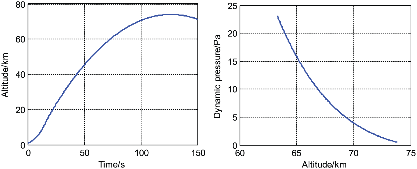
The trajectory and dynamic pressure of the ascend phase.

Considering the mission of the rocket, the deployment of the parachute is very important. Assuming the separation velocity between rocket and sonde is $10 m / s$ , the deployment process was simulated with a dynamic pressure of 20, 10, and 5 Pa, and at the apogee of the trajectory. The distance–time curve of the rocket and sonde for a dynamic pressure of 10 Pa is shown in Figure 9. Through the curve, we can determine that when the parachute was deployed, the distance was increasing first due to the separation velocity, the sonde closely approached the rocket under gravitational acceleration, and with the deployment of the parachute, drag forces worked on the sonde, causing the distance between the rocket and sonde to gradually increase.

Figure 9.

The distance between rocket and sonde after separation.

The characteristic parameters of the deployment under different conditions are listed in Table 1. From the table, we can determine that the minimum distance between the rocket and sonde increased with an increase in the deployment height and that inflation failure may result from increased times to deployment. Furthermore, as the dynamic pressure of the deployment increases, the deployment duration increases and the possibility of a rear-end collision also increases. The deployment condition should, therefore, be chosen with both sides considered.

Table 1.

Deployment situations under different conditions.

Deployment condition	Time (s)	Deploy time (s)	Minimum distance (m)
Dynamic pressure 20 Pa	81.4	2.4619	0.7472
Dynamic pressure 10 Pa	88.5	3.4341	2.6960
Dynamic pressure 5 Pa	95.7	5.1208	7.9060
Apogee	126.8	14.8537	Increases progressively

Results after wind compensation

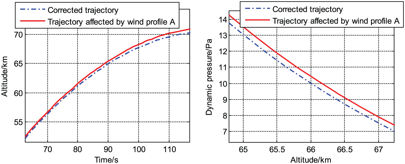
Based on the analysis and simulation results above, we chose the height with a dynamic pressure of 10 Pa as the separation point to deploy the parachute. With the goal of completing the mission, detecting the near-space environment, the dynamic pressure of 10 Pa was enacted to be at an altitude of 66 km, and in equation (28), $h_{0} = 66, 000$ and $h$ is the actual height that meets the dynamic pressure condition. Using the wind profiles we had from prior to the launch and performing some normalization processing, wind data at 32 points at the appointed altitudes were acquired. By running the program and using the simple software designed for wind compensation, the launch parameters can be updated, considering the wind effect. After a large number of simulations, the wind compensation results under different wind profiles are shown in Figures 10 –12.

Figure 10.

Wind compensation results for wind profile A.

Figure 11.

Wind compensation results for wind profile B.

Figure 12.

Wind compensation results for wind profile C.

In Figure 10, the trajectory affected by wind met the separation dynamic pressure at 66.158 km. After wind compensation, the altitude was 66.004 km, with an error of 4 m to the predetermined altitude, and the program ran for 2 min. In Figure 11, the trajectory affected by wind met the separation dynamic pressure at 66.585 km. After wind compensation, the altitude was 65.989 km, with an error of 11 m to the predetermined altitude, and the program ran for 3 min. In Figure 12, after compensation, the altitude changed from 66.464 to 65.995 km, and the program ran for almost 3 min. All the simulations were performed on a personal computer with an Intel Core i5 processor and random access memory of 4 GB, which is common in most computers. From the simulation times, we determined that the wind compensation method is suitable for calculating launch parameters immediately prior to launch. Due to the use of wind weighting, we can obtain approximate ranges of the launch parameters, which shorten the wind compensation time significantly, and the pattern search method is used to obtain precise solutions. Through the simulations, we determined that the errors were almost within 10 m.

With the simulations above, the wind compensation method has been verified to be rapid and precise.

Conclusion

This article has mainly analyzed the whole process dynamics of a sounding rocket, including motion on the launch rail, free flight phase, deployment of the parachute, inflation process, and steady descent. A high-precision dynamic model of a sounding rocket was built. The motions in each phase were investigated to study the entire trajectory of sounding rocket and sonde. Based on the dynamic model, a combination wind compensation method based on a 6-DoF dynamic model was presented to minimize the effects of wind and obtain the launch parameters, thus decreasing errors to almost 10 m.

Through the analysis, we studied the effects of sinking angle and sinking angle velocity on the trajectory. The lines-first deployment method and the inflation time method were used to study the deployment and inflation processes, and the relationships between deployment condition, deployment time, and the minimum distance between the rocket thrust stage and payload were obtained. Using the two-body dynamic model, the relative motion of the parachute–sonde system in the steady descent phase can be researched to further consider, for example, spin control. The wind compensation method combines wind weighting with the pattern search method, considering both efficiency and accuracy. The method was verified to be effective in this article.

Footnotes

Academic Editor: Crinela Pislaru

Declaration of conflicting interests

The author(s) declared no potential conflicts of interest with respect to the research,authorship,and/or publication of this article.

Funding

The author(s) disclosed receipt of the following financial support for the research,authorship,and/or publication of this article: This work was supported by the National Natural Science Foundation of China under the grant of 11272345.

References

Newell

HE.

Sounding rockets. New York: McGraw-Hill Education, 1959.

Emme

Bland

WM.

The history of rocket technology: essays on research, development, and utility. Detroit, MI: Wayne State University Press, 1964.

Arves

Jones

Kline

. Overview of hybrid sounding rocket program. In: Proceedings of the 33rd joint propulsion conference and exhibit, joint propulsion conferences, Seattle, WA, 06–09 July 1997. Reston, VA: AIAA.

Song

ZB.

The design of sounding rocket. Beijing, China: China Astronautic Publishing House, 1993.

Wang

KF.

Entering the Chinese space meteorological station. Scientist 2014; 8: 76–78.

Jiang

Liu

. Development status and trend of sounding rocket. Sci Technol Rev 2009; 27: 101–110.

Lazzarin

Bellomo

Barato

. SPONGE: a sounding rocket experiment for PMDs. In: Proceedings of the 48th AIAA/ASME/SAE/ASEE joint propulsion conference & exhibit, Atlanta, GA, 30 July–1 August 2012. Reston, VA: AIAA.

Casalino

Pastrone

Optimization of hybrid sounding rockets for hypersonic testing. J Propul Power 2012; 28: 405–411.

Zemcov

Smidt

Arai

. On the origin of near-infrared extragalactic background light anisotropy. Science 2014; 346: 732–735.

10.

Winebarger

Cirtain

Golub

. Discovery of finely structured dynamic solar corona observed in the Hi-C telescope. The Astrophys J Lett 2014; 787: L10.

11.

NASA sounding rockets annual report 2016. Wallops Island, VA: Sounding Rockets Program Office, 2017.

12.

Ceglia

Carey

Isakeit

. European User Guide to Low Gravity Platforms. UIC-ESAUM-0001 Issue 2 Revision 0, Erasmus User Centre and Communication Office ESA, 2005.

13.

Garcia

Yamanaka

SSC

Nogueira Barbosa

. VSB-30 sounding rocket: history of flight performance. J Aerosp Technol Manage 2011; 3: 325–330.

14.

Schütte

TEXUS and MAXUS preparations for the future. In: Proceedings of the 20th symposium on European rocket and balloon programmes and related research, Hyere, 22–26 May 2011, vol. 700, pp.503–507, http://spaceflight.esa.int/pac-symposium_archives/files/papers/s11_1schue.pdf

15.

Eerland

Box

Fangohr

. An open-source, stochastic, six-degrees-of-freedom rocket flight simulator with a probabilistic trajectory analysis approach. In: Proceedings of the AIAA modeling and simulation technologies conference, Grapevine, TX, 9–13 January 2017. Reston, VA: AIAA.

16.

Ewing

Bixby

Knacke

TW.

Recovery systems design guide. Gardena, CA: Irvin Industries Inc., 1978.

17.

Tang

Zhang

. Nine-degree-of-freedom model of bomb-parachute system. Acta Armamen 2007; 28: 449–452.

18.

Hoult

CP.

Sounding-rocket wind-response correction. J Spacecraft Rockets 2016; 53: 763–765.

19.

Duncan

Engebos

BF.

A rapidly converging iterative technique for computing wind compensation launcher settings for unguided rockets. White Sands Missile Range, NM: Atmospheric Sciences Laboratory, Army Electronics Command, 1969.

20.

Torczon

On the convergence of pattern search algorithms. SIAM J Optimiz 1997; 7: 1–25.