Integrating multiple adaptation results by utilization of support vector regression in case-based mechanical product design

Abstract

Case adaptation is crucial for a good and reasonable case-based design which is a common method in computer-aided design, because the solution of old case is not always the exact answer for the encountered new designing problem. Recently, a statistical feature-oriented adaptation method in the principle of k-nearest neighbors has been employed widely in case-based design because of its easily understandable mechanism for designers, but its adaptation accuracy is relatively low compared with knowledge-intensive method. This article presents a new method by integrating with multiple adaptation values from statistical feature-oriented adaptation methods to improve the adaptation accuracy. First, two simple statistical feature-oriented adaptation methods including mean and median approaches and other four statistical feature-oriented adaptation methods based on Euclidean distance, Manhattan distance, Gaussian transformation, and gray coefficient are used as individual statistical feature-oriented adaptation mode in this article, and each statistical feature-oriented adaptation method generates pre-adapting value under k-nearest neighbor. Then, support vector regression is utilized to make a combined adaptation which takes pre-adapting values as its inputs, and the new multiple statistical feature-oriented adaptation method integration based on support vector regression is named as MSFA-SVR. Furthermore, to validate the feasibility and superiority of MSFA-SVR, it was applied to the power transformer design and was compared with the classical statistical feature-oriented adaptation methods. Empirical comparison results indicated that MSFA-SVR achieves the better adaptation performance under k-nearest neighbor than other statistical feature-oriented adaptation methods in terms of adaptation accuracy.

Introduction

Supporting the design of new mechanical product by recalling past experiences and adapting them to the current design requirement is the long cherished desire of designers, as designers rely heavily on past design experiences in actual design, rather than designing everything from scratch. ¹ This kind of approach is known as case-based design (CBD), ² derived from the methodology of case-based reasoning (CBR). The concept of CBD focuses on the general idea of retaining a memory of previous design requirements and their solutions. It solves new problems by analogical reasoning on such retained information, ³ and the term ‘case’ captures representation of a previous problem-solving situation. However, real-world problems are dynamic and uncertain processes where idealistic modeling assumptions are rarely met. Accordingly, CBD has three challenging issues: (1) organization of case base, (2) case-retrieval technique, and (3) adaptation of past solutions to the current problem. Among these, the case adaptation has a significant effect on the success of CBD that plays a fundamental role in problem solving, because the solution in the retrieved case is not always appropriate for the encountered designing problem. However, most of the classic CBD systems are retrieval-only systems or act primarily as retrieval and reuse systems.^4,5 They merely perform adaptation process in the principle of 1-nearest neighbor (1-NN), namely, the solution of most similar case is the only candidate for new design problem, and the generation of new solution values heavily depends on human subjective judgement. ⁵ So, how to perform adaptation by reference to k similar cases without having to excessively rely on manual adaptation still remains as challenging obstacles to the CBD system.

To search for more accurate adaptation performance under k-NN, researchers of CBD in 1990s or so began to employ statistical feature-oriented adaptation (SFA) methods such as the closest analogy, ⁶ the equal mean (EM), ⁷ the median, ⁸ and weighted mean (WM). ⁹ Nowadays, they are also regarded as the baseline modes, whose advantages are the domain independence and easily to be implemented, but a potential drawback of CBD based on statistical adaptation is its low adaptation precision.^2,10,11 Moreover, the development of CBD-based intelligent techniques and soft computing has led mainly to two types of researches. One is intelligent feature-oriented adaptation (IFA) based on various machine learning models; the other is hybridization of intelligent techniques with statistical adaptation methods. Typical approaches for the first case are gene adaptation^12–17 and neuroadaptation.^18–22 For the second case, Huang et al. ¹³ and Qi et al. ²³ introduced the adjusting parameters in statistical adaptation models and used genetic algorithm and decision tree, respectively, to obtain the optimized adjusting parameters. Our previous work ²⁴ also adopted gray relational analysis to explore the hidden relational information in statistical adaptation model.

In fact, there is a belief in the area of computational intelligence that combining-modes system tends to minimize the disadvantages of single modes and maximize their advantages. ²⁵ This idea has already been applied into the area of financial analysis, ²⁶ housing value estimation, ¹⁰ cost prediction, ²⁷ and process determination^28,29 with satisfying results. Enlightened by these, this study presents a new methodology to improve the performance of SFA for case-based mechanical design, namely, integrating multiple adaptation results provided by independent statistical adaptation methods to the combined solution. Support vector regression (SVR), developed by Vapnik,^30,31 is utilized as a combiner to hybridize the results from different individual adaptation methods because of SVR’s good performance in combining scheme. ³² The contribution of this study is to take the advantages of SFA’s characteristics of easily being calculated and SVR’s characteristics of high generalization and propose a new multiple SFA integration based on SVR (MSFA-SVR) method, which is different from classical SFA and IFA studies. Furthermore, this research also investigates whether or not the proposed hybrid SFA adaptation method can produce higher performance than single SFA method. The next section gives a description on literature review of adaptation studies. Afterwards, the proposed MSFA-SVR method is discussed in detail in section “Specification on proposed method.” In section “Empirical comparison and discussion,” the empirical results are analyzed and discussed. Section “Conclusion” presents conclusion.

Research background

This section provides a brief introduction to the case adaptation in CBD, especially the statistical case adaptation. Several classical SFA methods are introduced in detail.

Case adaptation in CBD

When CBD systems are applied to real-world design problems, the retrieved design solutions can rarely be directly used as suitable solutions for a new problem. Retrieved solutions usually require a set of adaptations in order to be applied to new contexts. An adaptation can be considered as a situation/action pair. The situation contains the differences between the new and retrieved design requirements. The action captures the update for the retrieved design solution: solution components to be added, deleted, or changed ³³ or new feature values for the reused solution. ²¹ Accordingly, the case adaptation in CBD can be divided into two categories: component-oriented adaptation and feature-oriented adaptation. In early implementation of CBD, the most widely used form of adaptation strategy employs hand-coded adaptation rules, which demands a significant effort of knowledge acquisition for case adaptation.^15,34 When a new problem is presented to CBD system, it retrieves a similar case and sends it to the adaptation engine. The engine, in turn, selects an adaptation rule and starts a search in the memory for components able to substitute parts of the retrieved solution or for features able to modify values of the retrieved solution.

In this study, we focus on the feature-oriented adaptation in case-based mechanical design, as the parametric design is a common way for mechanical companies to rapidly develop new mechanical products within a short period of time, ³⁵ and designers are able to make a comparatively reasonable decision by inputting some easy-to-assess parameters into the parametric design system. However, the parametric design is a complex problem when there are massive parameters in the process of design, and the utilization of classical rule-based adaptation method in this situation demands a significant knowledge engineering effort to capture abundant adaptation rules. This prompted some studies to research machine learning–based adaptation under k-NN principle, and several learning methods have been employed in this area, for example, neural networks,^{19–22,36,37} SVR, ³⁸ genetic algorithm,^12,14–16 and partial-order planning. ³⁹ But insufficient knowledge badly affects the selection of an appropriate machine learning algorithm and its performance in feature-oriented adaptation.

An alternative to overcome these limitations in insufficient adaptation knowledge has been the use of a domain-independent statistical adaptation approach. So far, it has been employed widely in CBD system without considering the insufficient knowledge problem.^13,23,24 But, statistical adaptation deriving from techniques employed in standalone mode has been proven to be low adaptation accuracy compared with machine learning–based adaptation. ²³ As a combining mode system tends to minimize the disadvantages of single mode and maximize their advantages, it is worthwhile to combine several statistical adaptation results together to obtain the combined solution, such as the issue we intent to highlight and research in this article.

Statistical case adaptation research

The early algorithm of statistical adaptation used in the 90s is the mean method^6,7 and the median method. ⁸ Mean method is the average of the feature values of k-nearest neighbors (k-NNs), where k > 1. It is a classical measure of central tendency and treats all design cases as being equally influential on the feature-oriented adaptation. Median is the median of the feature values of k-NNs, where k > 2. It is another measure of central tendency and a more robust statistic when the number of cases increases. After that, an inverse distance weighted mean (IDWM) framework was developed, which allows more similar cases to have more influence than less similar ones. Suppose that there are k design cases retrieved from case base, and the hth (h ≤ k) case consists of design requirement part ${\mathit{x}}_h^R$ and solution part ${\mathit{x}}_h^S$ , while the new design requirement and solution values are represented as ${\mathit{x}\prime }^R$ and ${\mathit{x}\prime }^S$ , then the formula of IDWM is expressed by the following way ⁴⁰

$$x{\prime }_i^S=\sum _{h=1}^{h=k}\frac{1/1(\mu +\mathrm{dis}({\mathit{x}\prime }^R,{\mathit{x}}_h^R))(\mu +\mathrm{dis}({\mathit{x}\prime }^R,{\mathit{x}}_h^R))}{\sum _{i=1}^{i=k}1/1(\mu +\mathrm{dis}({\mathit{x}\prime }^R,{\mathit{x}}_h^R))(\mu +\mathrm{dis}({\mathit{x}\prime }^R,{\mathit{x}}_h^R))}{x}_{h·i}^S$$ (1)

where $x_{h·i}^S$ and $x{\prime }_i^S$ are the ith solution feature value of hth old case and new design, respectively, and $\mathrm{dis}({\mathit{x}\prime }^R,{\mathit{x}}_h^R)$ represents the distance value between requirement ${\mathit{x}\prime }^R$ and ${\mathit{x}}_h^R$ , and $\mu$ is a constant value. Furthermore, because of the imprecision and uncertainties of distance measurement in IDWM, a direct similarity weighted mean (DSWM) by substitution of the reciprocal of the similarity value into $\mathrm{dis}({\mathit{x}\prime }^R,{\mathit{x}}_h^R)$ calculation was developed by Qi et al., ²³ and the formula of DSWM can be expressed as follows

$$x{\prime }_i^S=\sum _{h=1}^{h=k}\frac{1/1(\mu \prime +\mathrm{sim}{({\mathit{x}\prime }^R,{\mathit{x}}_h^R)}^{-1})(\mu \prime +\mathrm{sim}{({\mathit{x}\prime }^R,{\mathit{x}}_h^R)}^{-1})}{\sum _{i=1}^{i=k}1/1(\mu \prime +\mathrm{sim}{({\mathit{x}\prime }^R,{\mathit{x}}_h^R)}^{-1})(\mu \prime +\mathrm{sim}{({\mathit{x}\prime }^R,{\mathit{x}}_h^R)}^{-1})}{x}_{h·i}^S$$ (2)

where $\mathrm{sim}({\mathit{x}\prime }^R,{\mathit{x}}_h^R)$ is the similarity between ${\mathit{x}\prime }^R$ and ${\mathit{x}}_h^R$ , which is inversely proportional to $\mathrm{dis}({\mathit{x}\prime }^R,{\mathit{x}}_h^R)$ , and $\mu \prime$ is a constant value and pre-defined as 0.5 in this article. Compared to the IDWM which only depends on distance metric, other similarity measurement approaches besides distance metric can be introduced in DSWM. It provides the possibility to improve the SFA’s accuracy. Thus, different statistical adaptation models can be constructed based on various similarity measurement approaches, according to equation (2). In this article, several similarity-related SFA methods using different similarity measurement metrics are adopted to generate the primary adaptation solutions. The details of these methods are described in the following section.

Specification on proposed method

This section makes specification on MSFA-SVR method. First, the framework of MSFA-SVR is illustrated. Then, the SVR for SFA integration is formulated in detail. Finally, an application example is given to show the feasibility of MSFA-SVR.

Framework of MSFA-SVR

The proposed adaptation integration is an approach to combine the adaptation results of different SFA methods to generate a joint adaptation, which is accomplished through the use of SVR. The new method is named as multiple statistical adaptation integration based on SVR (abbreviated as MSA-SVR). In MSFA-SVR, all the single SFA method are employed to solve the same adaptation task, and this article utilizes mean, ⁷ median, ⁸ Euclidean distance, ²³ Manhattan distance, ⁴⁰ Gaussian function, ²⁵ and gray coefficient degree ²⁵ to construct the six single SFA models, expressed as SFA-MA, SFA-ME, SFA-ED, SFA-MD, SFA-GF, and SFA-GC, respectively. Each SFA can generate pre-adapting values under k-NN, and then, these values are treated as inputs of SVR to make a secondary adaptation. The framework of MSFA-SVR is shown in Figure 1, where $x{\prime }_i^S(j)|(j=1,2,\dots ,6)$ are not only the pre-adaptation results of ith solution feature produced by six SFAs, but also the inputs of SVR. The mathematical formula is expressed in equation (2). $y_i$ is the final combined adaptation value for ith solution feature output by SVR model.

Figure 1.

Framework of the proposed MSFA-SVR.

Pre-adaptation results’ integration

The statistical adaptation methods are introduced in this section. The training sample of SVR and the mechanism of SVR for statistical adaptation integration are presented as well.

Independent statistic adaptation

As shown in Figure 1, this article puts forward independent SFA-MA, SFA-ME, SFA-ED, SFA-MD, SFA-GF, and SFA-GC to make pre-adaptation with k retrieved cases. Among them, SFA-ED, SFA-MD, SFA-GF, and SFA-GC adopt DSWM framework as shown in equation (2), but they use different similarity measurement metrics which are expressed in Table 1. In Table 1, g is the number of problem features of each case. For SFA-GF, $\mathrm{gau}(x{\prime }_i^R,x_{h·i}^R)$ expresses the transformation indicator between ${\mathit{x}\prime }^R$ and ${\mathit{x}}_h^R$ on ith requirement feature, and ${\sigma }_i$ is the flexure point. For SFA-GC, we suppose $[{\overline{\mathit{x}}}_h{]}^R$ is a requirement set of all old cases except for ${\mathit{x}}_h^R$ and ${\mathit{x}\prime }^R\in [{\overline{\mathit{x}}}_h{]}^R$ , $\mathrm{grey}(x{\prime }_i^R,x_{h·i}^R)$ is the gray coefficient degree of ith requirement feature between ${\mathit{x}\prime }^R$ and ${\mathit{x}}_h^R$ , and $\underset{i}{inf}|{[{\overline{\mathit{x}}}_h]}^R-x_{h·i}^R|$ and $\underset{i}{\sup }|{[{\overline{\mathit{x}}}_h]}^R-x_{h·i}^R|$ denote the minimum and maximum distance of ${\mathit{x}}_h^R$ and $[{\overline{\mathit{x}}}_h{]}^R$ , respectively.

Table 1.

Mechanisms of six statistical adaptation modes.

Similarity-related SFA method	Framework	Similarity measurement metric
SFA-ED	DSWM+Euclidean distance 23	$\mathrm{sim}({\mathbf{x}\mathbf{\text{'}}}^R,{\mathbf{x}}_h^R)=1-\left(\frac{1}{g}\sqrt{\sum _{i=1}^g{\left((x{\prime }_i^R-x_{h·i}^R)/(x{\prime }_i^R-x_{h·i}^R)\max (x{\prime }_i^R,x_{h·i}^R)\max (x{\prime }_i^R,x_{h·i}^R)\right)}^2}\right)$
SFA-MD	DSWM+Manhattan distance 40	$\mathrm{sim}({\mathbf{x}\mathbf{\text{'}}}^R,{\mathbf{x}}_h^R)=1-\left(\frac{1}{g}\sum _{i=1}^g|x{\prime }_i^R-x_{h·i}^R|/|x{\prime }_i^R-x_{h·i}^R|\max (x{\prime }_i^R,x_{h·i}^R)\max (x{\prime }_i^R,x_{h·i}^R)\right)$
SFA-GF	DSWM+Gaussian function 25	$\begin{array}{c}\mathrm{sim}({\mathbf{x}\mathbf{\text{'}}}^R,{\mathbf{x}}_h^R)=\sum _{i=1}^g{w}_j\mathrm{gau}(x{\prime }_i^R,x_{h·i}^R)\hfill \\ \mathrm{where}\mathrm{gau}(x{\prime }_i^R,x_{h·i}^R)=\exp [-{(\mathrm{dis}(x{\prime }_i^R,x_{h·i}^R)/\mathrm{dis}(x{\prime }_i^R,x_{h·i}^R)\sqrt{2}\times {\sigma }_i\sqrt{2}\times {\sigma }_i)}^2]\hfill \end{array}$
SFA-GC	DSWM+gray coefficient degree 25	$\begin{array}{c}\mathrm{sim}({\mathbf{x}\mathbf{\text{'}}}^R,{\mathbf{x}}_h^R)=\sqrt{\sum _{i=1}^g{\left(w_i\mathrm{grey}(x{\prime }_i^R,x_{h·i}^R)\right)}^2}\hfill \\ \mathrm{where}\mathrm{grey}(x{\prime }_i^R,x_{h·i}^R)=\frac{\underset{i}{\inf }|{\left[{\overline{\mathbf{x}}}_h\right]}^R-x_{h·i}^R|+\gamma \times \underset{i}{\sup }|{\left[{\overline{\mathbf{x}}}_h\right]}^R-x_{h·i}^R|}{\mathrm{dis}(x{\prime }_i^R,x_{h·i}^R)+\gamma \times \underset{i}{\sup }|{\left[{\overline{\mathbf{x}}}_h\right]}^R-x_{h·i}^R|}\hfill \end{array}$

SFA: statistical feature-oriented adaptation method; ED: Euclidean distance; MD: Manhattan distance; GF: Gaussian function; GC: gray coefficient degree; DSWM: direct similarity weighted mean.

Construction of training sample in SVR

After SFAs are implemented successfully, it is possible to utilize SVR to combine the six SFA modes. Pre-adaptations of independent SFAs for each solution feature could be treated as inputs of SVR, and the final adaptation result of the solution feature for new design requirement could be viewed as outputs of SVR. Thus, the new training sample set of the supervised learning of SVR is formed, and outputs of six independent SFAs are transformed as inputs of SVR through min–max normalization process. The mathematic formula is expressed as

$$\begin{array}{c}{\mathit{x}}_i=[x_i\left(1\right),x_i\left(2\right),x_i\left(3\right),x_i\left(4\right),x_i\left(5\right),x_i\left(6\right)]\hfill \\ x_i\left(j\right)=\frac{x{\prime }_i^S\left(j\right)-\mathrm{Min}\left(x{\prime }_i^S\left(j\right)\right)}{\mathrm{Max}\left(x{\prime }_i^S\left(j\right)\right)-\mathrm{Min}\left(x{\prime }_i^S\left(j\right)\right)}j=1,2,\dots ,6\hfill \end{array}$$ (3)

where ${\mathit{x}}_i$ is an input vector of SVR for ith solution feature adaptation. $x{\prime }_i^S(j)$ are the pre-adapting results of ith solution feature from SFA-MA, SFA-ME, SFA-ED, SFA-MD, SFA-GF, and SFA-GC. Let $y_i$ be the output value of SVR, namely, a final combined adaptation value of ith solution feature on the basis of ${\mathit{x}}_i$ , and then, the training sample set for SVR training could be expressed as $G=\{{\mathit{x}}_i,y_i\}(i=1,2,\dots ,p)$ , where ${\mathit{x}}_i\in R^6$ and $y_i\in R$ , and $p$ is the number of solution feature. For large-scale training data, another issue of training sample construction is to select a training subset (TS) which should extract maximum information from large dataset. Che et al. ⁴¹ pointed out that the trained SVR may be over-fitting when the training dataset is non-uniform (or imbalanced). To turn the imbalanced training dataset into a balanced data in the training phase, Che et al. ⁴¹ integrated the selection of TS and model for SVR and proposed a nested particle swarm optimization by inheriting the model selection of the existing TS-based SVR (TS-SVR). In this article, we pay close attention to the integration of multiple adaptation results from various SFA modes, and the proposed MSFA-SVR model is performed based on a small dataset. In future, we will try to introduce the selection of TS in MSFA-SVR for more complex design task with larger databases.

Mechanism of SVR for adaptation integration

The basic idea of SVR for SFA integration is to map the pre-adapting values into a higher dimensional space via a nonlinear mapping and then to do linear regression in this space with the unknown function in the following form: $f(x)={\mathit{w}}^T\phi ({\mathit{x}}_i)+b$ , where $\phi ({\mathit{x}}_i)$ is the high dimensional value space, nonlinearly mapped from the input space $\mathit{x}$ , and $\mathit{w}$ represents the normal vector and $b$ is the bias. They are estimated by minimizing the regularized risk function

$$R\left(C\right)=C\frac{1}{p}\sum _{i=1}^p{L}_{\epsilon }(y_i,f\left(x_i\right))+\frac{1}{2}\Vert \mathit{w}{\Vert }^2$$ (4)

$$L_{\epsilon }(y,f\left(x\right))=\{\begin{array}{c}\hfill |y-f\left(x\right)|-\epsilon |y-f\left(x\right)|\ge \epsilon \hfill \\ \multicolumn{1}{c}{0\mathrm{otherwise}}\end{array}$$ (5)

The first term $C(1/p)\sum _{i=1}^p{L}_{\epsilon }(y_i,f\left(x_i\right))$ in equation (4) is the empirical error, which are measured by $\epsilon$ -insensitive loss function^30,31 given by equation (5). The second term $(1/2)||\mathit{w}|{|}^2$ is the regularization term. $C$ is referred to as the regularized constant and it determines the trade-off between the empirical risk and the regularization term. $\epsilon$ is called the tube size and it is equivalent to the approximation accuracy placed on the training data. Both $C$ and $\epsilon$ are user-prescribed parameters.^42,43

To obtain the estimation of $\mathit{w}$ and $b$ , equation (4) is transformed to the primal function given by equation (6) by introducing the positive slack variables ${\xi }_i$ and ${{\xi }_i}^{*}$ as follows

$$\begin{array}{c}\underset{w,\xi ,{\xi }^{*}}{\mathrm{Min}}(\frac{1}{2}||\mathit{w}|{|}^2+C\sum _{i=1}^p({\xi }_i+{{\xi }_i}^{*}))\hfill \\ \mathrm{s}.\mathrm{t}.\{\begin{array}{c}\hfill y_i-({\mathit{w}}^T\phi ({\mathit{x}}_i)+b)\le \epsilon +{\xi }_i\hfill \\ \multicolumn{1}{c}{({\mathit{w}}^T\phi ({\mathit{x}}_i)+b)-y_i\le \epsilon +{{\xi }_i}^{*}}\\ \multicolumn{1}{c}{{\xi }_i,{{\xi }_i}^{*}\ge 0i=1,2,\dots ,p}\end{array}\hfill \end{array}$$ (6)

Finally, by introducing the Lagrange multipliers and exploiting the optimality constraints, the decision function $f(x)$ has the following explicit form ³⁰

$$f(x,{\alpha }_i,{\alpha }_i^{*})=\sum _{i=1}^p({\alpha }_i-{\alpha }_i^{*})K(\mathit{x},{\mathit{x}}_i)+b$$ (7)

In equation (7), ${\alpha }_i$ and ${\alpha }_i^{*}$ are the so-called Lagrange multipliers. They satisfy the equalities ${\alpha }_i\times {\alpha }_i^{*}=0$ , ${\alpha }_i\ge 0$ and ${\alpha }_i^{*}\ge 0$ , and are obtained by maximizing the dual function of equation (6) which has the following form

$$\begin{array}{cc}\multicolumn{1}{c}{R({\alpha }_i,{\alpha }_i^{*})=}& \sum _{i=1}^p{y}_i({\alpha }_i-{\alpha }_i^{*})-\epsilon \sum _{i=1}^p({\alpha }_i+{\alpha }_i^{*})\hfill \\ -\frac{1}{2}\sum _{i=1}^p\sum _{j=1}^p({\alpha }_i-{\alpha }_i^{*})({\alpha }_j-{\alpha }_j^{*})K(x_i,x_j)\hfill \end{array}$$ (8)

with the following constraints

$$\sum _{i=1}^p({\alpha }_i-{\alpha }_i^{*})=0,0\le {\alpha }_i\le C,0\le {\alpha }_i^{*}\le C,i=1,2,\dots ,p$$

Based on the Karush–Kuhn–Tucker (KKT) conditions of the quadratic programming, only a number of coefficients $({\alpha }_i-{\alpha }_i^{*})$ in equation (7) will assume non-zero values. The input points associated with them could be named as support vectors; among them the points with $|{\alpha }_i-{\alpha }_i^{*}|=C$ are called error support vectors, as they are lying outside the boundary of the adaptive model, and the input points with $0<|{\alpha }_i-{\alpha }_i^{*}|<C$ are referred to as non-error support vectors, because they exactly lie on the boundary of the predictive model, and the number of non-error support vectors is $q$ .

Implementation of MSFA-SVR

An application example of MSFA-SVR is presented in this section to illustrate the procedure of hybrid statistical adaptation.

Application example

In this study, a total of 55 power transformer cases from S1, S2, S3, and S4 series with eight requirement features (R1–R8) and four solution features (F1–F4) are selected to construct MSFA-SVR model as listed in Table 2 and Appendix 1 (Table 10). Actually, how to determine the representative features of design cases and remove irrelevant ones is an important issue during the real SFA process. Feature selection (FS) technique is crucial for large-sized design case in SFA to strengthen the adaptation efficiency and accuracy by eliminating redundant features. Recently, many related data-driven FS methods have been proposed. Chakraborty and Pal ⁴⁴ utilized neural networks to conduct two connectionist FS schemes that able to simultaneously select the useful features and learn the relationships between input and output features. Che et al. ⁴⁵ presented a novel mutual information FS method based on the normalization of the maximum relevance and minimum common redundancy (N-MRMCR-MI) which shows superior performance by comparing with other state-of-art FS algorithms. Our previous studies^46,47 also tried to use neighborhood rough set algorithm to obtain the minimal set of features and extracted the hidden relationships between problem and solution features of design cases. In this example, to simplify this implementation, we select small-size power transformer case (R1–R8 problem features and F1–F4 solution features) without applying FS method. Among R1–R8, R8 (connection symbol (CS)) belongs to non-numerical feature, so 0–1 textual similarity measure metric ⁴⁸ is applied to figure the similarity, that is, 1 means two symbolic values are same, otherwise 0. For other numerical features (R1–R7 and F1–F4), min–max normalization is applied to scale all data into the range of [0,1], which helps SFA and SVR to improve the calculation performance. The formula of min–max normalization is given by equation (3). We implement the proposed method using support vector machine (SVM) toolbox available in MATLAB R2008b environment.

Table 2.

Requirement and solution features of the power transformer case.

Requirement features			Solution features
Variable	Feature	Unit	Variable	Feature	Unit
R1	Rated capacity (RC)	kV A	F1	Armature diameter (AD)	mm
R2	Primary voltage (PV)	kV	F2	Insulation radius (IR)	mm
R3	Secondary voltage (SV)	kV	F3	Coil radial thickness (CRT)	mm
R4	No-load loss (NL)	kW	F4	Wire cross section (WCS)	mm2
R5	Load loss (LL)	kW
R6	No-load current (NC)	A
R7	Impedance voltage (IV)	kV
R8	Connection symbol (CS)	Null

SVR model construction

Inspired by the empirical findings,^49–51 radial basis kernel $\exp (-\gamma ||x_i-x_j|{|}^2)$ is used as the kernel function of MSFA-SVR because of its good performance under the general smoothness assumptions. Following previous SVR studies,^38,42,43,52 the performance of SVR is insensitive to $\epsilon$ , and the reasonable values of $\epsilon$ are 0.01. Meanwhile, two parameters should be tuned to construct SVR model, that is, $C$ and $\gamma$ . For $C$ and $\gamma$ , it is not known beforehand which values of $C$ and $\gamma$ are the best for one problem, where $C$ determines the trade-offs between minimizing fitting errors and minimizing model complexity. Currently, some kinds of parameter search approaches are employed such as cross-validation via parallel grid search, heuristics search, and inference of model parameters within the Bayesian evidence framework. For median-sized problems, cross-validation might be the most reliable way for model parameter selection.^49,50 In v-fold cross-validation, the training set is first divided into v subsets. In the ith (i = 1, 2, …, v) iteration, the ith set (validation set) is used to estimate the performance of the SVR trained on the remaining (v – 1) sets (training set). The performance is generally evaluated by mean absolute percentage error (MAPE). The final performance of SVR is evaluated by average MAPE of v folds subsets. In grid-search process, pairs of $(C,\gamma )$ are tried and the one with the best cross-validation accuracy is picked up, and they could be searched in the ranges of $[2^{-5},2^{-3},\dots ,2^{13},2^{15}]$ and $[2^{-15},2^{-13},\dots ,2^1,2^3]$ . In this study, we prefer a grid search on $(C,\gamma )$ using 10-fold cross-validation, and we implement this optimization process under 9-NN with 55 example cases to find the optimal solution. Results of $(C,\gamma )$ via grid search and 10-fold cross-validation are shown in Table 3, from which we can find that $(2^9,2^{-7})$ is the best one.

Table 3.

Results of SVR parameters via grid search and 10-fold cross-validation.

C	γ
	2−15	2−13	2−11	2−9	2−7	2−5	2−3	2−1	21	23
2−5	24.24%	24.24%	24.24%	24.24%	24.24%	24.24%	24.24%	24.24%	24.24%	24.24%
2−3	24.24%	24.24%	24.24%	24.24%	24.24%	24.24%	24.24%	24.24%	24.24%	24.24%
2−1	24.24%	24.24%	24.24%	24.24%	24.24%	24.24%	24.24%	24.24%	24.24%	24.24%
21	24.24%	24.24%	24.24%	24.24%	24.24%	21.21%	21.21%	22.40%	19.80%	19.80%
23	24.24%	24.24%	24.24%	24.24%	21.21%	21.21%	21.21%	22.40%	19.80%	19.80%
25	24.24%	24.24%	21.21%	19.70%	21.21%	19.70%	19.80%	21.21%	19.80%	19.80%
27	24.24%	21.21%	21.21%	18.18%	18.18%	19.70%	19.80%	19.70%	19.70%	19.80%
29	21.21%	21.21%	19.70%	18.18%	16.67%	18.18%	19.80%	19.70%	19.70%	19.80%
211	21.21%	19.70%	19.70%	18.40%	18.18%	18.18%	19.80%	18.18%	18.18%	19.80%
213	21.21%	19.70%	18.18%	18.40%	20.80%	18.40%	21.21%	18.40%	20.80%	21.21%
215	21.21%	18.18%	18.18%	20.80%	20.80%	18.40%	21.21%	18.40%	20.80%	22.40%

SVR: support vector regression.

SFA results integration

According to Table 2, the initial solution feature values can be figured out using SFA-MA, SFA-ME, SFA-ED, SFA-MD, SFA-GF, and SFA-GC, as shown in Table 7. Then, the adaptive results of each independent SFAs are also considered as inputs of SVR (represented as X_AD, X_IR, X_CRT, X_WCS) under the framework of MSFA-SVR. After that, in terms of the ready-built SVR model and the handbook of power transformer design, the solution feature values for the new design requirement can be obtained. For simplicity, this study implements MSFA-SVR under 5-NN and employs ED metric to select the similar cases. The results of application example including the new design requirements for R1–R8 features, five design cases with highest similarities, feature adaptation results of SFAs and final adaptation values produced by MSFA-SVR are listed in Appendix 2.

Empirical comparison and discussion

This section focuses on the comparison of adaptation ability of the examined methods in terms of adaptation accuracy. Some discussions are presented based on empirical results, considering different k-NNs.

Objective and comparative methods

The objective of this empirical comparison is to compare the adaptation abilities of the proposed method and other SFA methods. The experimental design is shown in Figure 2.

Figure 2.

Experimental design.

Two types of classic SFAs, namely, simple SFA (i.e. SFA-MA and SFA-ME) and similarity-related SFA (i.e. SFA-ED, SFA-MD, SFA-GF, and SFA-GC), are employed as comparative methods to perform the empirical comparison. Furthermore, we would like to investigate the performances of MSFA-SVR under different numbers of design cases. Therefore, the adaptation performance of MSFA-SVR would not only be compared with its opponents but also be compared inside MSFA-SVR under 1-NN, 3-NN, 5-NN, 7-NN, 9-NN, and 11-NN.

Testing data and evaluation

In addition to the 55 cases mentioned above, other 30 power transformer cases are applied to compose testing data listed in Appendix 1 (Table 11). So, there are three types of data employed in the empirical comparison of MSFA-SVR, that is, training data, validating data, and testing data. Training data are used to train SFAs, validating data are used to determine the parameters of SFAs, while testing data are used as unseen data, and leave-one-out cross-validation is utilized to assess the performances of adaptation. Every time one case was selected from testing data in order as a testing case, the requirement feature values of testing case were considered as the new requirement problem and its corresponding solution feature values were used to compare with the adaptation results produced by adaptive modes. So, there were 30 empirical results in this empirical comparison. To compare the performances, this article employed the MAPE ³⁸ and the root mean square error (RMSE) ⁵³ as measurements of derivation between actual and adapted values. Compared with mean absolute error, MAPE can be utilized to measure the relative error (0–1) of adaptation computation by normalizing the error calculation. RMSE displays the variance of predicted adaptation for candidate adaptation methods in terms of millimeter. They are formulated as

$$\begin{array}{c}\mathrm{MAP}{E}_i=\frac{1}{30}\sum _{j=1}^{30}\frac{|e{v}_{\mathrm{ij}}-a{v}_{\mathrm{ij}}|}{a{v}_{\mathrm{ij}}}\hfill \\ \mathrm{RMS}{E}_i=\sqrt{\frac{1}{30}\sum _{j=1}^{30}{(e{v}_{\mathrm{ij}}-a{v}_{\mathrm{ij}})}^2}\hfill \end{array}$$ (9)

where $a{v}_{\mathrm{ij}}$ and $e{v}_{\mathrm{ij}}$ are the actual value and adaptation value for ith feature in jth empirical comparison. Moreover, we used the analysis of variance (ANOVA) test to determine whether the statistically significant differences exist among the comparative methods in out-of-sample adaptation. To further identify the significant differences between any two methods, Tukey’s honesty significant different (HSD) test^54,55 was used in this experiment to compare all pairwise differences simultaneously.

Results

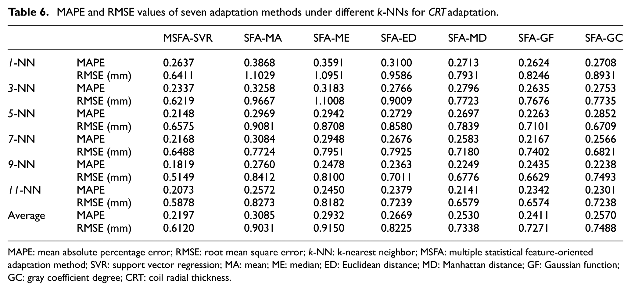
First, to compare the adaptive performances of MSFA-SVR, SFA-MA, SFA-ME, SFA-ED, SFA-MD, SFA-GF, and SFA-GC, the MAPE and RMSE values of such adaptation methods under 1-NN, 3-NN, 5-NN, 7-NN, 9-NN, and 11-NN for four solution features (AD, IR, CRT, and WCS) adaptation are listed in Tables 4–7. Second, to abstract the changes of performances of MSFA-SVR with different k values, the adapted solution values for testing case generated by MSFA-SVR in 30 times leave-one-out cross-validation and the corresponding real values of testing case are depicted in Figures 3–6. Furthermore, to determine the statistical differences of performance measures among seven adaptation methods for each k-NN principle and solution feature adaptation, we carried out the ANOVA and Tukey’s HSD tests, and the corresponding results are described in Tables 8 and 9. In Table 9, we rank the seven methods from 1 (the best) to 7 (the worst) to show the comparison results more clearly.

Table 4.

MAPE and RMSE values of seven adaptation methods under different k-NNs for AD adaptation.

		MSFA-SVR	SFA-MA	SFA-ME	SFA-ED	SFA-MD	SFA-GF	SFA-GC
1-NN	MAPE	0.2429	0.3528	0.3483	0.3490	0.3141	0.3132	0.3013
	RMSE (mm)	70.5124	89.8069	88.7262	83.8339	77.6269	77.1500	76.6122
3-NN	MAPE	0.2293	0.3055	0.3047	0.3210	0.3027	0.2826	0.2746
	RMSE (mm)	66.0450	85.7146	87.9315	79.4248	74.8583	66.6742	73.7546
5-NN	MAPE	0.2071	0.2877	0.2852	0.2847	0.2575	0.2363	0.2412
	RMSE (mm)	67.1949	80.5878	79.1096	72.5425	73.5039	70.8732	66.8765
7-NN	MAPE	0.2020	0.2520	0.2376	0.2456	0.2430	0.2291	0.2387
	RMSE (mm)	64.4766	79.5055	78.1561	77.1859	73.1018	73.8988	72.8135
9-NN	MAPE	0.1809	0.2398	0.2419	0.2206	0.2311	0.2183	0.2118
	RMSE (mm)	60.0170	81.7150	74.6261	76.4647	73.5329	73.9143	71.4657
11-NN	MAPE	0.1822	0.2389	0.2367	0.2262	0.2144	0.2091	0.2040
	RMSE (mm)	62.0734	80.4224	78.1751	70.0256	70.4146	75.2069	72.3946
Average	MAPE	0.2074	0.2795	0.2757	0.2745	0.2605	0.2481	0.2453
	RMSE (mm)	65.0532	82.9587	81.1208	76.5796	73.8397	72.9529	72.3195

MAPE: mean absolute percentage error; RMSE: root mean square error; k-NN: k-nearest neighbor; AD: armature diameter; MSFA: multiple statistical feature-oriented adaptation method; SVR: support vector regression; MA: mean; ME: median; ED: Euclidean distance; MD: Manhattan distance; GF: Gaussian function; GC: gray coefficient degree.

Table 5.

MAPE and RMSE values of seven adaptation methods under different k-NNs for IR adaptation.

		MSFA-SVR	SFA-MA	SFA-ME	SFA-ED	SFA-MD	SFA-GF	SFA-GC
1-NN	MAPE	0.2431	0.3504	0.3217	0.2969	0.3064	0.2412	0.2888
	RMSE (mm)	30.7642	40.8828	38.4470	36.8432	32.0718	30.3875	29.5828
3-NN	MAPE	0.2180	0.3278	0.3045	0.2804	0.2741	0.2733	0.2774
	RMSE (mm)	26.4198	38.9208	40.0977	28.3552	25.1151	23.4841	30.3402
5-NN	MAPE	0.2249	0.3074	0.2639	0.2435	0.2519	0.2247	0.2481
	RMSE (mm)	26.5750	34.9965	37.9394	30.1840	29.6580	24.3680	27.2735
7-NN	MAPE	0.2240	0.2774	0.2992	0.2723	0.2471	0.2416	0.2406
	RMSE (mm)	26.1469	36.5992	36.2285	27.0671	29.4046	22.3506	27.6974
9-NN	MAPE	0.1870	0.2936	0.2521	0.2275	0.2142	0.2349	0.2149
	RMSE (mm)	24.2353	39.0044	33.5520	32.5907	34.7565	31.6168	28.0265
11-NN	MAPE	0.1997	0.2420	0.2222	0.2306	0.2229	0.2082	0.2122
	RMSE (mm)	26.7316	31.4714	32.2891	32.1960	27.4033	27.3314	22.7013
Average	MAPE	0.2161	0.2998	0.2772	0.2585	0.2528	0.2373	0.2470
	RMSE (mm)	26.8121	36.9792	36.4256	31.2060	29.7349	26.5897	27.6036

MAPE: mean absolute percentage error; RMSE: root mean square error; k-NN: k-nearest neighbor; AD: armature diameter; MSFA: multiple statistical feature-oriented adaptation method; SVR: support vector regression; MA: mean; ME: median; ED: Euclidean distance; MD: Manhattan distance; GF: Gaussian function; GC: gray coefficient degree; IR: insulation radius.

Table 6.

MAPE and RMSE values of seven adaptation methods under different k-NNs for CRT adaptation.

		MSFA-SVR	SFA-MA	SFA-ME	SFA-ED	SFA-MD	SFA-GF	SFA-GC
1-NN	MAPE	0.2637	0.3868	0.3591	0.3100	0.2713	0.2624	0.2708
	RMSE (mm)	0.6411	1.1029	1.0951	0.9586	0.7931	0.8246	0.8931
3-NN	MAPE	0.2337	0.3258	0.3183	0.2766	0.2796	0.2635	0.2753
	RMSE (mm)	0.6219	0.9667	1.1008	0.9009	0.7723	0.7676	0.7735
5-NN	MAPE	0.2148	0.2969	0.2942	0.2729	0.2697	0.2263	0.2852
	RMSE (mm)	0.6575	0.9081	0.8708	0.8580	0.7839	0.7101	0.6709
7-NN	MAPE	0.2168	0.3084	0.2948	0.2676	0.2583	0.2167	0.2566
	RMSE (mm)	0.6488	0.7724	0.7951	0.7925	0.7180	0.7402	0.6821
9-NN	MAPE	0.1819	0.2760	0.2478	0.2363	0.2249	0.2435	0.2238
	RMSE (mm)	0.5149	0.8412	0.8100	0.7011	0.6776	0.6629	0.7493
11-NN	MAPE	0.2073	0.2572	0.2450	0.2379	0.2141	0.2342	0.2301
	RMSE (mm)	0.5878	0.8273	0.8182	0.7239	0.6579	0.6574	0.7238
Average	MAPE	0.2197	0.3085	0.2932	0.2669	0.2530	0.2411	0.2570
	RMSE (mm)	0.6120	0.9031	0.9150	0.8225	0.7338	0.7271	0.7488

MAPE: mean absolute percentage error; RMSE: root mean square error; k-NN: k-nearest neighbor; MSFA: multiple statistical feature-oriented adaptation method; SVR: support vector regression; MA: mean; ME: median; ED: Euclidean distance; MD: Manhattan distance; GF: Gaussian function; GC: gray coefficient degree; CRT: coil radial thickness.

Table 7.

MAPE and RMSE values of seven adaptation methods under different k-NNs for WCS adaptation.

		MSFA-SVR	SFA-MA	SFA-ME	SFA-ED	SFA-MD	SFA-GF	SFA-GC
1-NN	MAPE	0.2504	0.3328	0.3231	0.2980	0.2936	0.2673	0.2818
	RMSE (mm)	6.5877	10.4130	9.6162	9.3667	9.8566	9.0979	9.3900
3-NN	MAPE	0.2301	0.2952	0.2775	0.2773	0.2857	0.2729	0.2571
	RMSE (mm)	7.6287	9.7712	9.0672	9.7726	9.3755	8.3820	8.7981
5-NN	MAPE	0.2144	0.2851	0.2676	0.2659	0.2646	0.2559	0.2596
	RMSE (mm)	7.2604	9.2031	8.5918	8.6808	8.7281	8.0375	7.7597
7-NN	MAPE	0.2076	0.2528	0.2529	0.2802	0.2529	0.2317	0.2393
	RMSE (mm)	6.6634	8.9423	8.2578	8.1863	8.3857	7.7867	7.6345
9-NN	MAPE	0.1838	0.2702	0.2488	0.2497	0.2422	0.2460	0.2628
	RMSE (mm)	6.1268	8.3884	8.2898	8.0906	8.1236	7.8116	8.3419
11-NN	MAPE	0.2129	0.2261	0.2184	0.2186	0.2324	0.2048	0.2121
	RMSE (mm)	7.3986	9.1455	8.8629	8.3169	8.5900	7.9974	7.8058
Average	MAPE	0.2166	0.2771	0.2647	0.2650	0.2619	0.2464	0.2521
	RMSE (mm)	6.9443	9.3106	8.7809	8.7356	8.8433	8.1855	8.2883

MAPE: mean absolute percentage error; RMSE: root mean square error; k-NN: k-nearest neighbor; MSFA: multiple statistical feature-oriented adaptation method; SVR: support vector regression; MA: mean; ME: median; ED: Euclidean distance; MD: Manhattan distance; GF: Gaussian function; GC: gray coefficient degree; WCS: wire cross section.

Table 8.

ANOVA test results for hold-out sample.

k-NN	ANOVA test
	AD		IR		CRT		WCS
	Statistics F	p value	Statistics F	p value	Statistics F	p value	Statistics F	p value
1-NN	23.452	0.000*	15.734	0.000*	16.357	0.000*	21.456	0.001*
3-NN	22.465	0.000*	8.714	0.001*	17.345	0.000*	20.435	0.000*
5-NN	17.467	0.001*	11.690	0.000*	9.356	0.001*	18.456	0.000*
7-NN	11.563	0.000*	8.132	0.001*	10.346	0.000*	11.387	0.000*
9-NN	13.235	0.001*	13.251	0.000*	16.223	0.000*	12.456	0.000*
11-NN	25.678	0.000*	7.388	0.000*	10.567	0.000*	24.465	0.001*

k-NN: k-nearest neighbor; ANOVA: analysis of variance; AD: armature diameter; IR: insulation radius; CRT: coil radial thickness; WCS: wire cross section.

*

The mean difference among the six adaptation methods is significance at the 0.05 level.

Table 9.

Comparison results with ranked comparative methods for hold-out sample.

	Ranks of methods
	1		2		3		4		5		6		7
AD
1-NN	MSFA-SVR	<*	SFA-GC	<*	SFA-MD	<	SFA-GF	<*	SFA-ME	<	SFA-ED	<*	SFA-MA
3-NN	MSFA-SVR	<*	SFA-GC	<*	SFA-GF	<*	SFA-MD	<*	SFA-ME	<	SFA-MA	<*	SFA-ED
5-NN	MSFA-SVR	<*	SFA-GF	<*	SFA-GC	<*	SFA-MD	<	SFA-ED	<*	SFA-ME	<*	SFA-MA
7-NN	MSFA-SVR	<*	SFA-GF	<*	SFA-GC	<*	SFA-ME	<*	SFA-MD	<*	SFA-ED	<	SFA-MA
9-NN	MSFA-SVR	<*	SFA-GC	<	SFA-GF	<*	SFA-ED	<*	SFA-MD	<*	SFA-MA	<*	SFA-ME
11-NN	MSFA-SVR	<*	SFA-GF	<*	SFA-GC	<*	SFA-MD	<*	SFA-ED	<*	SFA-ME	<	SFA-MA
IR
1-NN	SFA-GF	<	MSFA-SVR	<*	SFA-GC	<*	SFA-ED	<	SFA-MD	<*	SFA-ME	<*	SFA-MA
3-NN	MSFA-SVR	<*	SFA-GF	<	SFA-MD	<	SFA-GC	<*	SFA-ED	<*	SFA-ME	<*	SFA-MA
5-NN	SFA-GF	<	MSFA-SVR	<*	SFA-GC	<	SFA-ED	<*	SFA-MD	<*	SFA-ME	<*	SFA-MA
7-NN	MSFA-SVR	<*	SFA-GC	<	SFA-GF	<*	SFA-MD	<*	SFA-ED	<	SFA-MA	<*	SFA-ME
9-NN	MSFA-SVR	<*	SFA-MD	<	SFA-GC	<*	SFA-ED	<*	SFA-GF	<*	SFA-ME	<*	SFA-MA
11-NN	MSFA-SVR	<*	SFA-GF	<*	SFA-GC	<*	SFA-ME	<	SFA-MD	<*	SFA-ED	<*	SFA-MA
CRT
1-NN	SFA-GF	<	MSFA-SVR	<*	SFA-GC	<	SFA-MD	<*	SFA-ED	<*	SFA-ME	<*	SFA-MA
3-NN	MSFA-SVR	<*	SFA-GF	<*	SFA-GC	<	SFA-ED	<*	SFA-MD	<*	SFA-ME	<*	SFA-MA
5-NN	SFA-GF	<	SFA-GF	<*	SFA-GC	<*	SFA-MD	<*	SFA-ED	<*	SFA-ME	<	SFA-MA
7-NN	SFA-GF	<	MSFA-SVR	<*	SFA-GC	<	SFA-MD	<*	SFA-ED	<*	SFA-ME	<*	SFA-MA
9-NN	MSFA-SVR	<*	SFA-GF	<*	SFA-GC	<	SFA-MD	<*	SFA-ED	<*	SFA-ME	<*	SFA-MA
11-NN	MSFA-SVR	<*	SFA-MD	<*	SFA-GC	<*	SFA-GF	<	SFA-ED	<*	SFA-ME	<*	SFA-MA
WCS
1-NN	MSFA-SVR	<*	SFA-GF	<*	SFA-GC	<*	SFA-MD	<	SFA-ED	<*	SFA-MA	<	SFA-ME
3-NN	MSFA-SVR	<*	SFA-GC	<*	SFA-GF	<*	SFA-ED	<*	SFA-MD	<	SFA-ME	<*	SFA-MA
5-NN	MSFA-SVR	<*	SFA-GF	<	SFA-GC	<*	SFA-MD	<	SFA-ED	<*	SFA-ME	<*	SFA-MA
7-NN	MSFA-SVR	<*	SFA-GF	<*	SFA-GC	<*	SFA-ME	<*	SFA-MD	<*	SFA-MA	<	SFA-ME
9-NN	MSFA-SVR	<*	SFA-MD	<	SFA-GF	<*	SFA-GC	<*	SFA-ED	<	SFA-ME	<*	SFA-MA
11-NN	SFA-GF	<	SFA-GC	<	MSFA-SVR	<*	SFA-MD	<*	SFA-ED	<	SFA-ME	<*	SFA-MA

AD: armature diameter; MSFA: multiple statistical feature-oriented adaptation method; SVR: support vector regression; MA: mean; ME: median; ED: Euclidean distance; MD: Manhattan distance; GF: Gaussian function; GC: gray coefficient degree; NN: nearest neighbor; SFA: statistical feature-oriented adaptation method; IR: insulation radius; CRT: coil radial thickness; WCS: wire cross section.

*

The mean difference among the six adaptation methods is significance at the 0.05 level.

Figure 3.

The adapted AD values and real values of testing case generated by MSFA-SVR in 30 times leave-one-out.

Figure 4.

The adapted IR values and real values of testing case generated by MSFA-SVR in 30 times leave-one-out.

Figure 5.

The adapted CRT values and real values of testing case generated by MSFA-SVR in 30 times leave-one-out.

Figure 6.

The adapted WCS values and real values of testing case generated by MSFA-SVR in 30 times leave-one-out.

Discussion

This section analyzes the comparative results from three perspectives, including comparison between MSFA-SVR and other SFAs, comparison inside MSFA-SVR, and comparison of adaptation difference.

Comparison between MSFA-SVR and other SFAs

Tables 4–7 show the MAPE and RMSE values of four solution feature (AD, IR, CRT, and WCS) adaptation achieved by MSFA-SVR, SFA-MA, SFA-ME, SFA-ED, SFA-MD, SFA-GF, and SFA-GC with different k-NNs. Taking the average MAPE and RMSE indices of all k-NNs into account, MSFA-SVR achieves better adaptation performance than other SFA methods, because of its relative lower average MAPE and RMSE values of four solution feature adaptation. Among classical SFAs methods, SFA-GF marginally outperforms SFA-GC and SFA-MD and significantly outperforms SFA-ED, SFA-ME, and SFA-MA. This means that the performances of similarity-related SFAs (SFA-ED, SFA-MD, SFA-GF, and SFA-GC) are better than those of simple SFA (SFA-ED and SFA-MD). However, the minor differences of adaptation performance among SFA-MD, SFA-GF, and SFA-GC demonstrate that the improvement of adaptation performance is insignificant only changing the similarity measurement metrics. So, it is a meaningful attempt to probe into new adaptation model from the point of view of SFA integration, as this article has done. However, the larger MAPE and RMSE values of comparative methods under 1-NN, 3-NN, and 5-NN indicate that there are several noises and uncertainties, so it is necessary to select more training cases and data pre-processing to help the statistical adaptation methods improve the adaptation performance. Furthermore, for MSFA-SVR, as it contains several similarity measurement metrics and SVR algorithms, which results in having more parameters than other SFAs, we also need additional example data to optimize these parameters to improve the stability of MSFA-SVR results.

Comparison inside MSFA-SVR with various k-NN

Figures 3-6 show the adapted solution values generated by MSFA-SVR under various k-NNs and the corresponding real values of test cases. As mentioned above, in each time of leave-one-out cross-validation, the requirement feature values of one testing case were considered as the new requirement problem and its corresponding solution feature values were used to compare with the adaptation results produced by adaptive modes. From Figures 3 to 6, we can find that MSFA-SVR under 1-NN achieves the lowest adaptive performance among all MSFA-SVR models. This phenomenon provides some evidences on the assumption that adaptation performance of 1-NN is sensitive to noise and is not robust, because only the most similar case is selected to generate the adapted value. In general, the MSFA-SVR with larger k could produce more accurate adapted results which are much closer to the real data, as shown the adapted values of MSFA-SVR under 1-NN, 3-NN, 5-NN, 7-NN, and 9-NN. However, when k is larger than 10, several irrelevant cases with related lower similarities could also be selected, which result in the fluctuations of adaptive performances. For example, MSFA-SVR under 11-NN generates large deviation data when S3-200 is test case in Figure 3, S3-330 is test case in Figure 4, S2-500 is test case in Figure 5, and S2-10000 is test case in Figure 6. Moreover, the MAPE and RMSE values of MSFA-SVR under 11-NN in four solution adaptation experiments, that is, (0.1822, 62.0734 mm, AD adaptation), (0.1997, 26.7316 mm, IR adaptation), (0.2073, 0.5878 mm, CRT adaptation) and (0.2129, 7.3986 mm, WCS adaptation), are also larger than those of MSFA-SVR under 9-NN, that is, (0.1809, 60.0170 mm, AD adaptation), (0.1870, 24.2353 mm, IR adaptation), (0.1819, 0.5149 mm, CRT adaptation) and (0.1838, 6.1268 mm, WCS adaptation), as listed in Tables 9–12. In a word, considering the MAPE and RMSE indices, the suitable value of k for MSFA-SVR is 9.

Comparison of adaptation difference

Beside MAPE and RMSE indices, we also performed an ANOVA procedure to determine whether the statistically significant differences exist among the seven comparative methods under each k-NN principle in the hold-out sample. All of the ANOVA results listed in Table 8 are significant at the 0.05 level, suggesting that there are significant differences among all comparative methods. To further identify the significant difference between any two methods, Tukey’s HSD test was used to compare all pairwise differences simultaneously at the 0.05 level in this comparison. Table 9 summarizes the results of Tukey’s HSD test, from which we can find that when MSFA-SVR in all four feature adaptation experiments is treated as the testing target, the mean difference between the two adjacent methods are significant at the 0.05 level (with the exception of the 1-NN and 5-NN in IR adaptation; 1-NN, 5-NN, and 7-NN in CRT adaptation and 11-NN in WCS adaptation), indicating that the MSFA-SVR performs the best in most adaptation tasks. Table 9 also shows that simple SFA methods (SFA-ME and SFA-MA) achieve the poor performances at a 95% statistical confident level, which explains the relative low performance of simple statistical case adaptation.

Conclusion

To improve the adaptation performances of classic SFAs, this article presents a hybrid adaptation method called as MSFA-SVR. In MSFA-SVR, six SFAs generate pre-adapting values under k-NN principle, and these values are further integrated by SVR to make a combined adaptation. To describe the possibilities of the methodology, the proposed method is applied to power transformer design. Moreover, the empirical comparisons are carried out to validate the superiority of MSFA-SVR. From the view of design example and comparison test, we can draw the conclusion that MSFA-SVR achieves the better performance compared with classical single SFAs. In future, we try to upgrade the proposed hybrid adaptation method from the following aspects. First, this study mainly concerns the comparison between MSFA-SVR and classical statistic adaptation methods. We will make more comparisons on adaptation performances between MSFA-SVR and other IFA methods based on pure SVR, neural networks, genetic algorithm, and so on. Besides adaptation accuracy, the computational cost will be another criterion for comparison between MSFA-SVR and IFA methods. Second, as the parameter configuration could influence the performance of MSFA-SVR, we will try to introduce new optimization methods such as artificial immune algorithm, ⁵⁶ simulated annealing, ⁵⁷ and firefly algorithm^54,58 into MSFA-SVR to determine the $\epsilon$ , $C$ , $\gamma$ , and k values automatically, instead of manual trial-and-error way. Third, as we mentioned in section “Application example,” how to select useful features is an important issue for SFA, specially for large-sized design case. Likewise, MSFA-SVR system could be suffered from the disturbances of irrelevant features in real situation. So, we will apply FS technique in MSFA-SVR to avoid these disturbances in future. Finally, in this study, the experimentation is performed using a small power transformers dataset, so we will build MSFA-SVR model on the basis of larger databases which contain hundreds or thousands of cases and analyze its applicability in more complex design task.