Sage Journals: Discover world-class research

Abstract

The work presented in this article constitutes a contribution to modeling and forecasting the demand in a food company, by using time series approach. Our work demonstrates how the historical demand data could be utilized to forecast future demand and how these forecasts affect the supply chain. The historical demand information was used to develop several autoregressive integrated moving average (ARIMA) models by using Box–Jenkins time series procedure and the adequate model was selected according to four performance criteria: Akaike criterion, Schwarz Bayesian criterion, maximum likelihood, and standard error. The selected model corresponded to the ARIMA (1, 0, 1) and it was validated by another historical demand information under the same conditions. The results obtained prove that the model could be utilized to model and forecast the future demand in this food manufacturing. These results will provide to managers of this manufacturing reliable guidelines in making decisions.

Keywords

Demand forecasting time series autoregressive integrated moving average (ARIMA)

Introduction

In today’s competitive manufacturing environment, and to respond quickly to shifting demand, organizations are moving toward a more effective demand-driven supply chain. The market has evolved into a “pull” environment with customers more demanding and discriminating, dictating to the supplier what products they desire and when they need them delivered.¹

Demand forecasting is crucial to inventory management. Inventory stock levels depend on demand’s forecasts. In fact, inaccurate estimation of demand can cause significant costs to pay, which proves that the process is not improved. Consequently, many systems incur large investments in inventories to avoid “stock outs.” A further complicating issue is that some demands can be intermittent demands, which means that there is a time when we have no demand and other time when we have successive demands. Intermittent demands present many difficulties for traditional statistical demand forecasting methods.

Generally, there are many approaches to forecast demand among which we find the exponential smoothing, for example. But, when applying these approaches, we need to have historical data. In the beginning, there is no information about the past, we use then an estimation based on similar cases or engineer’s experiences. In this case, we have a big amount of uncertainty which will be avoided with time.

For most organizations, managing demand is challenging because of the difficulty in forecasting future consumer needs accurately.¹ More than 74 % of the responds in a research survey, shows the poor forecasting accuracy and demand volatility as the increasing major challenges to supply chain flexibility.² Best performing companies tend to improve supply chain flexibility, agility, and responsiveness through improving forecasting accuracy throughout the long supply chain.² The managers in these companies must link forecasting to improvement goals and use past performance to avoid past errors and then reach a high level of efficiency.³

Researchers came out with much work in the forecasting domain and suggested many methods among which we find two principal approaches much utilized: time series approaches and artificial neural network (ANN) techniques.

ANN models have been successfully involved in forecasting demand. These models are characterized by intervals with considerable variation of demand. ANN approach is considered as an alternative when it comes to the ability to capture the nonlinearity in data set.

ANN is applied in different fields. Gaafar and Choueiki⁴ applied a neural network model to a lot-sizing problem as a part of material requirements planning for the case of deterministic time-varying demand.⁵

To compare ANN and ARIMA method and to assess the performance of the two methods, a study related to electricity demand has been done by Prybutok et al.⁶ to forecast a time series. ANN seems to be outperformed. Another study was done by Ho et al.⁷ using simulated failure time of a compressor to determine the more accurate forecasting model. The two methods are used to forecast the failure of the system.⁸

Aburto and Weber⁹ combined the two forecasting methods which are ARIMA and neural networks. The efficiency of the hybrid model is compared with traditional forecasting methods.¹⁰

This brief review of the literature shows that ANN is a strength tool aiming at the modeling of any time series. Nevertheless, in our article, we will test the ARIMA model at first to prove its ability to make accurate forecasts in the food company as a priori study.

In our article, we are interested the most in the time series approach: autoregressive integrated moving average (ARIMA) models,^11

–14 multivariate transfer function models,^11,15 dynamic models,¹¹ and generalized autoregressive conditional heteroskedasticity (GARCH) models¹⁶ have also been proposed. Certainly, ARCH and GARCH models are increasingly utilized and are considered as important tools in the analysis of time series data, especially in the case of financial applications. But, they are specifically dedicated to the analysis and forecasting of volatility which is not our aim in this current article.

In all sectors, demand forecasts are of great importance. Indeed, predicting the demand facilitates the decision on the amount to produce and thus on the supply of the raw material and inventory management. In our case, we will work in a food company—which requires more than in other sectors—forecasts that are very reliable and accurate as long as it will affect the production of perishable goods. Besides, products in a food company having steady predictable demand need efficient supply chains that shorten lead times and support limited inventory.

A robust supply chain management system requires the presence of managers who are aware of the necessity of collaboration between different functions: planning, procurement, manufacturing, and logistics. Let’s take the example of the collaboration of planning function with suppliers. Over time, we feed our database to build a history that will be used to make our forecasts. After developing our model, which is the purpose of our article, we will easily have the planned application transmitted to the planning function. The latter carries out its production plan related to suppliers.

The aim is therefore to devise an optimal production plan based on accurate forecasts to minimize the total production cost composed by the procurement, processing, storage, and distribution costs. Expected benefits from these forecasts are reduced inventories, lower supply chain costs, increased return on assets, greater customer satisfaction, and reduced lead times. However, this optimal production plan should meet different company constraints among others: production capacity, minimum production lots, and so on.

We will be interested in the evolution by making forecasts of the demand in a Moroccan food company. To achieve its objectives, the company must rely on precise forecasts. In this context, our article aims mainly to study the demand to provide precise forecasts and to respect the permissible error margin. The main idea is that forecasting accuracy drives the performance of inventory management.

The aim of the present study is the modeling and forecasting of demand by using Box–Jenkins time series approach, especially the ARIMA. To achieve this goal, we used large and consistent historical demand data: from January 2010 until December 2015. Several ARIMA models were developed and evaluated by four performance criteria: Akaike criterion (AIC), Schwarz Bayesian criterion (SBC), maximum likelihood, and standard error. The adequate model was validated by new historical demand data under the same conditions. In this article, the second section presents a literature review about demand forecasting studies. The third section is consecrated to the results and discussions of our case study. Finally, the article concludes with a summary and the future work.

Literature review

Forecasting demand

In today’s organizations, which are subject to abrupt and enormous changes that affect even the most established of structures and where all requirements of business sector need accurate and practical reading into future, the forecasts are becoming very crucial since they are the sign of survival and the language of business in the world. A forecast is a science of estimating the future level of some variables. The variable is most often demand, but it can also be something else, such as supply or price.¹⁷ Forecasting is the operation of making assumption about the future values of studied variables.¹⁸

In manufacturing, forecasting demands is among the most crucial issues in inventory management¹⁹; it can be used in various operational planning activities during the production process: capacity planning, used-product acquisition management.²⁰

For both types of supply chain processes “push/pull,” the demand forecasts are considered the ground of supply chain’s planning. The pull processes in the supply chain are realized with reference to customer demand, while all push processes are realized in anticipation of customer demand.²¹ A company must take into consideration such factors before selecting a suitable forecasting methodology because the choice of a methodology is not as simple as it seems. Forecasting methods are categorized according to four types: qualitative, time series, causal, and simulation.²¹

A time series is nothing but observations according to the chronological order of time.¹⁷ Time series forecasting models use mathematical techniques that are based on historical data to forecast demand. It is founded on the hypothesis that the future is an expansion of the past; that’s why we can definitely use historical data to forecast future demand.¹

Many studies about demand forecasting by time series analysis have been done in several domains. They encircle demand forecasting for food product sales,²² tourism,²³ maintenance repair parts,^19,24 electricity,^25,26 automobile,²⁷ and some other products and services.^28,29,30

By time series analysis, the forecasting accuracies depend on the characteristics of time series of demand. If the transition curves show stability and periodicity, we will reach high forecasting accuracies, whereas we can’t expect high accuracies if the curves contain highly irregular patterns.²⁷

Autoregressive integrated moving average

To model time series, we can work with the traditional statistical models including moving average, exponential smoothing, and ARIMA. These models are linear since the future values are cramped to be linear functions of past data.

During the past few decades, researchers have been focusing much on linear models since they had proved simplicity in comprehension and application.

Time series forecasting models are mostly used to predict demand. Under an autoregressive moving average hypothesis, Kurawarwala and Matsuo³¹ calculated the seasonal variation of demand by using historical data and validated the models by examining the forecast performance. Miller and Williams³² mixed seasonal factors in their model to improve forecasting accuracy, the seasonal factors are calculated from multiplicative model. Hyndman³³ widened Miller and Williams’³² work by applying different relationships between trend and seasonality under seasonal ARIMA hypothesis. The classical ARIMA approach becomes prohibitive, and in many cases, it is impossible to determine a model, when seasonal adjustment order is high or its diagnostics fail to indicate that time series is stationary after seasonal adjustment. In such cases, the static parameters of the classical ARIMA model are considered the principal constraint to forecasting high variable seasonal demand. Another constraint of the classical ARIMA approach is that it requires a large number of observations to determine the best fit model for a data series.

An ARIMA model is labeled as an ARIMA model (p, d, q), wherein:

p is the number of autoregressive terms;

d is the number of differences; and

q is the number of moving averages.

The autoregressive process

Autoregressive models assume that Y_t is a linear function of the preceding values and is given by equation (1)

Y_{t} = α_{1} Y_{t - 1} + ε_{t}

Literally, each observation consists of a random component (random shock, ε) and a linear combination of the previous observations. α₁ in this equation is the self-regression coefficient.

The integrated process

The behavior of the time series may be affected by the cumulative effect of some processes. For example, stock status is constantly modified by consumption and supply, but the average level of stocks is essentially dependent on the cumulative effect of the instantaneous changes over the period between inventories. Although short-term stock values may fluctuate with large contingencies around this average value, the level of the series over the long term will remain unchanged. A time series determined by the cumulative effect of an activity belongs to the class of integrated processes. Even if the behavior of a series is erratic, the differences from one observation to the next can be relatively low or even oscillate around a constant value for a process observed at different time intervals. This stationarity of the series of differences for an integrated process is a crucial characteristic viewed from the statistical analysis side of the time series. Integrated processes are the archetype of nonstationary series. A differentiation of order 1 assumes that the difference between two successive values of Y is constant. An integrated process is defined by equation (2)

Y_{t} = Y_{t - 1} + ε_{t}

where the random perturbation ε_t is a white noise.

The moving average process

The current value of a moving averaging process is a linear combination of the current disturbance with one or more previous perturbations. The moving average order indicates the number of previous periods embedded in the current value. Thus, a moving average is defined by equation (3)

Y_{t} = ε_{t} - θ_{1} ε_{t - 1}

Box and Jenkins³⁴ was founded on the contributions of Yule³⁵ and Wold³⁶ to develop a practical approach in order to perform ARIMA models. The Box–Jenkins principle consists of three iterative steps of model identification, parameter estimation, and diagnostic checking steps³⁷. The principle rule to identify the model is that if a time series is obtained from an ARIMA process, it should have some theoretical autocorrelation properties. By matching the theoretical and empirical autocorrelation patterns, we make it possible to identify one or several potential models for the given time series. Box and Jenkins³⁴ proposed to use the autocorrelation function (ACF) and the partial autocorrelation function (PACF) of the sample data as the basic tools to identify the order of the ARIMA model.

As far as the identification step is concerned, we should produce a stationary time series, which is a required condition to find the ARIMA model, so, we mostly need data transformation. The statistical characteristics of a stationary time series such as the mean and the autocorrelation structure are constant over time. We usually need to apply differencing and power transformation to the data to remove the trend and stabilize the variance before an ARIMA model can be fitted.

After that, it becomes easy to calculate the model parameters and then specify the model. These parameters are estimated so that the overall error is reduced.

Finally, we move to the diagnostic checking of model adequacy. In this last step, we make sure that the hypothesis we made about the errors are contended. The diagnostic statistics and plots of residuals can be used to assess the adequacy of future values to our data. If the model is not adequate, we have to make other estimation of parameters followed by the model validation. Diagnostic information can help us come up with new models.

Box–Jenkins model constitutes a process approach to follow and repeat till reaching a high degree of satisfaction about the model and having reduced errors. Consequently, we can freely use this model to forecast our variable.

Researchers approve that the estimation of parameters requires a large number of observations. Consequently, there are some limits for using ARIMA model. Nevertheless, once we apply ARIMA model, we reach a high quality in the opposite of the time series models.

Results and discussion

In this article, the demand forecasting of the final product in a food manufacturing is conducted based on real data, and the accuracy and characteristics are studied. This study examines the effectiveness of demand forecasting in a food manufacturing.

Based on the Box–Jenkins approach, our study will be carried out in three parts: identification, estimation, and verification. The model shown in Figure 1 is based on the demand of the final product in a Moroccan food manufacturing from January 2010 until December 2015.

Figure 1.

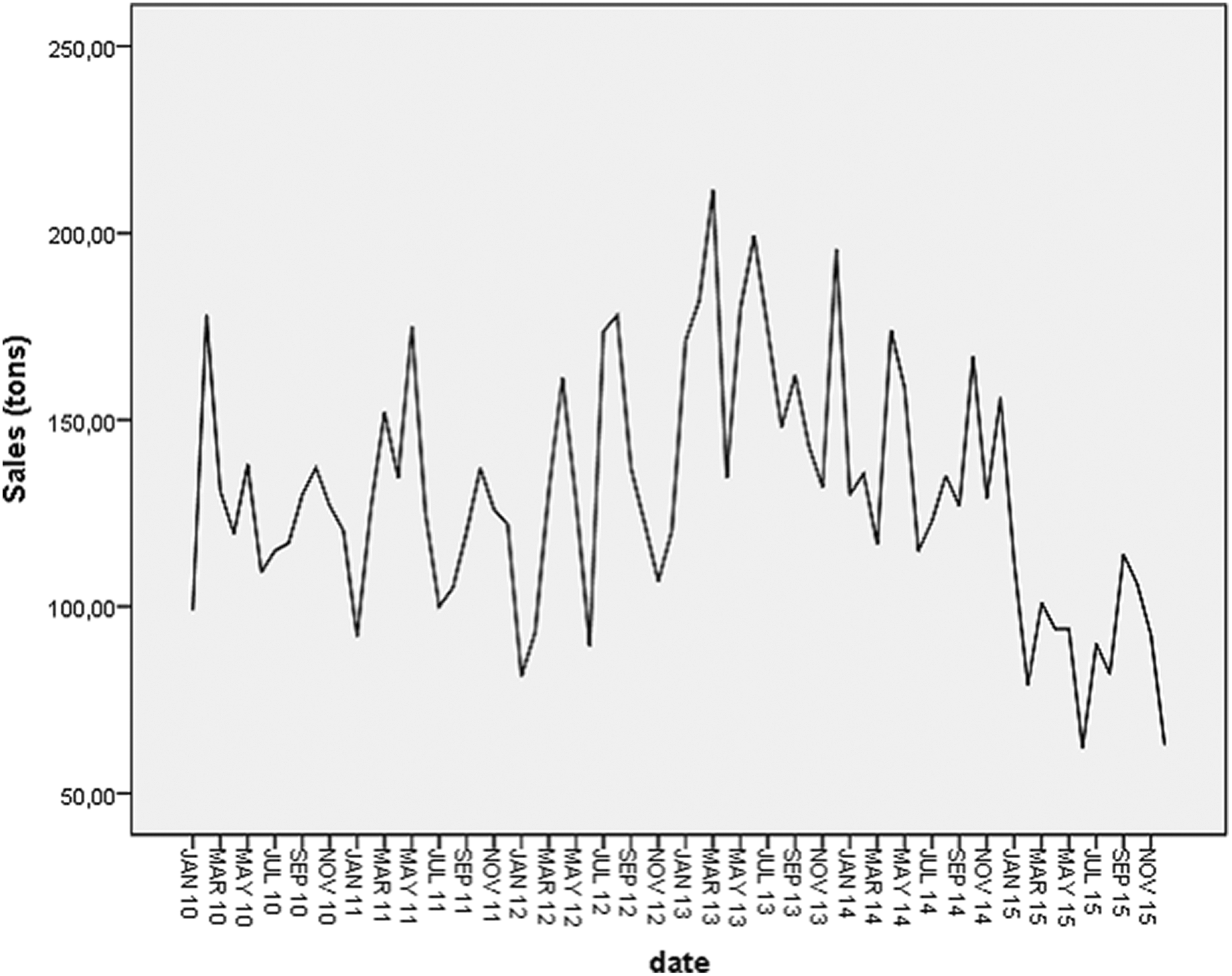
Evolution of the final product’s sales.

Identification of model

In this step, we start with the initial preprocessing of the data to make it stationary, and then we choose possible values of p and q which we can of course adjust as model fitting progresses.

For stationarity, the series shown in Figures 2 and 3, respectively, fluctuates around an average value and its ACF decays to zero fairly rapidly which proves the stationarity of the time series.

Figure 2.

ACF correlograms of the demand series. ACF: autocorrelation function.

Figure 3.

PACF correlograms of the demand series. PACF: partial autocorrelation function.

Moreover, to assess whether the data come from a stationary process we can perform the unit root test: Dickey–Fuller test for stationarity. After carrying out the test on the Xlstat software, the results are grouped in Table 1.

H₀: The series has a unit root.

H₁: The series does not have a unit root. The series is stationary.

Table 1.

Test results.

τ (observed value)	−1.350
τ (critical value)	−0.717
p Value (unilateral)	0.844
α	0.05

Since the calculated p value is greater than the threshold significance level α = 0.05, the null hypothesis H₀ cannot be rejected. The risk of rejecting the null hypothesis H₀ while it is true is 84.38%.

In our case, and after verification of the stationarity of the series, we notice from the ACF and PACF correlograms that our model is not pure AR or pure MA. We therefore tested several models to identify the most suitable one for sales.

Estimation of model’s coefficients

The ARIMA procedure of the SPSS time series module³⁸ allows estimating the coefficients of the models that we have previously identified by providing the parameters p, q, and d, using a fast maximum likelihood estimation algorithm.^39

–42

The execution of the procedure adds new time series representing the values adjusted or predicted by the model, residuals (adjustment errors) and confidence intervals of the adjustment at a 95% confidence level. The best model is as simple as possible and minimizes certain criteria, namely AIC, SBC, variance and maximum likelihood.^43
–45 The chosen model is that of ARIMA (0, 1, 1). For the other models, either Student “T-RATIO” test values are found in the range ±1.96, or one of the values of the minimization criteria is higher than that found for the ARIMA model (1, 0, 1) with the constant value.

Table 2 summarizes the values of the different models and proves the choice of the model on which we will base our predictions. It is clear from Table 2 that the ARIMA model (1, 0, 1) is selected because all the coefficients are significantly different from 0 according to the Student test (|T-RATIO| ≥ 1, 96) with an acceptable level of adjustment.

Table 2.

Coefficients of different models.

Models/Characteristics		ARIMA (1, 0, 2)	ARIMA (2, 0, 2)	ARIMA (1, 0, 1)	ARIMA (1, 0, 0)	ARIMA (0, 0, 1)	ARIMA (1, 0, 1) without constant
AR (1)	α ₁	0.92913	0.71371	0.90792	0.49434	−0.41704	0.99755623
	SEB	0.104616	0.761758	0.094852	0.1074471	0.1119989	0.00444769
	T value	8.8813204	0.9369292	9.571955	4.600820	−3.723567	224.28617
	p Value	0.00000000	0.35216008	0.00000000	0.00001823	0.00039384	0.0000000
MA (1)	θ ₁	0.52269	0.31779	0.63880			0.71392452
	SEB	0.167073	0.741595	0.161531			0.08579173
	T value	3.1284995	0.4285186	3.954655			8.32160
	p Value	0.00258711	0.66964815	0.00018319			0.0000000
AR (2)	α ₂		0.19759
	SEB		0.659442
	T value		0.2996279
	p Value		0.76538859
MA (2)	θ ₂	0.17062	0.30202
	SEB	0.142258	0.409353
	T value	1.1993429	0.7377864
	p Value	0.23455708	0.46322050
Constant	Cte	124.42969	124.52640	125.53260	128.53887	129.22650
	SEB	12.608189	12.601296	11.785537	6.5715235	4.8971088
	T value	9.8689581	9.8820312	10.651411	19.559981	26.388326
	p Value	0.00000000	0.00000000	0.00000000	0.00000000	0.00000000
AIC		688.86593	690.82312	688.77347	689.37103	693.59055	692.04831
SBC		697.9726	702.20645	695.60347	693.92437	698.14388	696.60164
Log likelihood		−340.43297	−340.41156	−341.38674	−342.68552	−344.79527	−344.02415
Error		28.034898	28.221721	28.214812	28.576249	29.443759	28.461048

SBC: Schwarz Bayesian criterion; AIC: Akaike criterion; ARIMA: autoregressive integrated moving average; SEB: Standard Error of B (B: Regression Coefficient).

The model residue is stationary and follows a white noise process in the range of ±40. The residue histogram shows whether the distribution of residues approximates a normal distribution. In our case, we have residues that distribute relatively normal around zero and with a relatively low dispersion at a 5% risk.

The chosen model parameters are presented in Table 3.

Table 3.

ARIMA model parameters.

				Estimate	SE	t
Sales (tons)-Model_1	No transformation	Constant		125.524	12.466	10.069
		AR	Lag 1	0.908	0.095	9.537
		MA	Lag 1	0.639	0.162	3.938

ARIMA: autoregressive integrated moving average.

The developed model is given by equation (4)

y_{t} = δ + α_{1} y_{t - 1} - θ_{1} ε_{t - 1} + ε_{t}

with:

y_t , y_t−1: sales of period t and t−1, respectively.

$ε_{t}, ε_{t - 1}$ : residuals of period t and t−1, and constitute a white nose.

α₁, θ₁: coefficients of autoregressive and moving average processes, respectively.

From Table 3, we can extract the coefficients of autoregressive and moving average processes. Therefore, equation (4) becomes as follows

y_{t} = 125.524 + 0.90792 y_{t - 1} - 0.6388 ε_{t - 1}

Accuracy of ARIMA (1, 0, 1) model

The accuracy of the developed model was evaluated by comparing the experimental and the simulated sales in the same period. Figure 4 reports this comparison and reveals that the selected model has a high accuracy and ability to simulate the dynamic behavior of sales. Therefore, this model can be used to analyze and model the demand in this food manufacturing.

Figure 4.

Sales, fit, LCL, and UCL. LCL: lower control limit; UCL: upper control limit.

From the graph, we notice that the model is validated since the predicted demand fluctuates around the fit. We also note that the predicted demand stayed between the upper limit and the lower limit.

We can see that the error variates but it is among the tolerance interval. In order to minimize this error, we propose a new approach in our future work.

Forecast

After we have defined the most appropriate model of demand in our case, we have to make the forecasting; to do this and so to predict trends and develop forecast, we used the IBM SPSS Forecasting. Table 4 and Figure 5 present the results of the sales forecasts that we obtained by applying our model ARIMA (1, 0, 1) for the next 10 months from January 2016 to October 2016.

Table 4.

Forecast sales from January 2016 to October 2016.

Model		73	74	75	76	77	78	79	80	81	82
Sales-Model_1	Forecast	95.12	97.92	100.46	102.77	104.86	106.77	108.49	110.06	111.49	112.78
	UCL	151.41	156.21	160.35	163.95	167.08	169.83	172.25	174.38	176.26	177.93
	LCL	38.83	39.63	40.57	41.59	42.64	43.70	44.74	45.75	46.71	47.63

LCL: lower control limit; UCL: upper control limit.

Figure 5.

Sales, fit, LCL, UCL, and forecasting. LCL: lower control limit; UCL: upper control limit.

We can clearly see that the model chosen can be used for modeling and forecasting the future demand in this food manufacturing, but each time we need to feed the historical data with the new data to enrich it in order to improve the new model and forecasting.

The forecasts obtained after modeling facilitated the decision on the production in this food company. In fact, the model enabled us to forecast the demand and make accurate predictions. Once we obtain a demand forecast, it will be much easier end very clear to make the right production planning and thus eliminate big cost losses. That will help us take right decisions related to supplying raw materials and determination of daily production. Moreover, that will affect the whole production process eliminating then any kind of loss.

Conclusion

Demand forecasting is an important function of managing supply chain. Its integration with other business functions makes it one of the most important planning processes business can deploy for future. In this context, we developed an ARIMA model to model the demand forecasting of the finished product in a food manufacturing by using Box–Jenkins time series approach. The historical demand data were used to develop several models and the adequate one was selected according to four performance criteria: SBC, AIC, standard error, and maximum likelihood. The model that we selected and which minimizes the four previous criteria is ARIMA (1, 0, 1). The results obtained proves that this model can be used for modeling and forecasting the future demand in this food manufacturing; these results will provide to managers of this manufacturing reliable guidelines in making decisions. As future work, we will develop other models by using a combination of qualitative and quantitative techniques to generate reliable forecasts and increase the forecast accuracy. We will also try neural network approach to compare it with ARIMA’s results in order to confirm the ANN’s strength in the food company. Furthermore, we will make an ARIMA-radial basis function (RBF) combination always to achieve the same goal: high accuracy.

Footnotes

Declaration of Conflicting Interests

The authors declared no potential conflicts of interest with respect to the research,authorship,and/or publication of this article.

Funding

The authors received no financial support for the research,authorship,and/or publication of this article.

ORCID iD

Zineb Aman

References

Wisner

Tan

Leong

. Principles of supply chain management: a balanced approach. Mason: Thomson South-Western, 2011.

Dawei

. Fundamentals of supply chain management. Bookboon.com, 2011. www.bookboon.com (accessed 15 March 2017). ISBN: 978-87-7681-798-5.

Baker

Hart

. The marketing book, 7th ed. Amsterdam: Elsevier, 2016. Print ISBN: 9780415703765/10.4324/9781315890005.

Gaafar

Choueiki

. A neural network model for solving the lot-sizing problem. Omega 2000; 28(2): 175–184.

Sustrova

. An artificial neural network model for a wholesale company’s order-cycle management. Int J Eng Bus Manage 2016; 8: 2.

Prybutok

Mitchell

. Comparison of neural network models with ARIMA and regression models for prediction of Houston’s daily maximum ozone concentrations. Eur J Oper Res 2000; 122(1): 31–40.

Xie

Goh

. A comparative study of neural network and Box-Jenkins ARIMA modeling in time series prediction. Comput Ind Eng 2002; 42(2–4): 371–375.

Kandananond

. A comparison of various forecasting methods for autocorrelated time series. Int J Eng Bus Manage 2012; 4: 4.

Aburto

Weber

. Improving supply chain management based on hybrid demand forecasts. Appl Soft Comput 2007; 7(1): 136–144.

10.

Mitrea

Lee

CKM

. A comparison between neural networks and traditional forecasting methods: a case study. Int J Eng Bus Manage 2009; 1: 11.

11.

Doulai

Cahill

. Short-term price forecasting in electric energy market. In: Proceedings of international power engineering conference, (organisers, Nanyang Technical University, et al.), Grand Copthorne Waterfront, Singapore, 17–19 May 2001, pp. 749–754. IEEE.

12.

Contreras

Espinola

Nogales

. ARIMA models to predict next-day electricity prices. IEEE Trans Power Syst 2003; 18(3): 1014–1020.

13.

Conejo

Plazas

Espinola

. Day-ahead electricity price forecasting using the wavelet transform and ARIMA models. IEEE Trans Power Syst 2005; 20(2): 1035–1042.

14.

El Bahi

Ezzine

Aman

. Modeling and forecasting of fuel selling price using time series approach: case study. In: Proceedings of the international conference on control decision and information technologies, Thessaloniki, Greece, 10–13 April 2018. IEEE.

15.

Nogales

Conejo

. Electricity price forecasting through transfer function models. J Oper Res Soc 2006; 57(4): 1–7.

16.

Garcia

Contreras

Van Akkeren

. A GARCH forecasting model to predict day-ahead electricity prices. IEEE Trans Power Syst 2005; 20(2): 867–874.

17.

Bozarth

Handfield

. Introduction to operations and supply chain management, 4th ed. Raleigh: North Carolina State University, 2016.

18.

Tsay

. Time series and forecasting: brief history and future research. J Am Stat Assoc 2000; 95: 638–643.

19.

Ghobbar

Friend

. Evaluation of forecasting methods for intermittent parts demand in the field of aviation: a predictive model. Comput Oper Res 2003; 30: 2097–2114.

20.

Toktay

. Forecasting product returns. In: Guide

VDR

Jr van Wassenhove

(eds) Business aspects of closed-loop supply chains. Pittsburgh: Carnegie Mellon University Press, 2003.

21.

Chopra

Meindl

. Supply chain management. Strategy, planning & operation. In: Das summa summarum des management. Gabler, 2007, pp. 265–275.

22.

Miller

McCahon

Miller

. Foodservice forecasting with simple time series models. J Hosp Tour Res 1991; 14: 9–21.

23.

Song

. Tourism demand modeling and forecasting—a review of recent research. Tour Manage 2008; 29: 203–220.

24.

Willemain

Smart

Schwarz

. A new approach to forecasting intermittent demand for service parts inventories. Int J Forecast 2004; 20: 375–387.

25.

Taylor

de Menezes

McSharry

. A comparison of univariate methods for forecasting electricity demand up to a day ahead. Int J Forecast 2006; 1: 1–16.

26.

Weron

. Electricity price forecasting: a review of the state-of-the-art with a look into the future. Int J Forecast 2014; 30: 1030–1081.

27.

Mitsutaka

Akira

. Examination of demand forecasting by time series analysis for auto parts remanufacturing. J Remanuf 2015; 5: 1. DOI: 10.1186/s13243-015-0010-y.

28.

Gardner

Jr . Exponential smoothing: the state of the art—part II. Int J Forecast 2006; 22: 637–666.

29.

Liu

Wang

. Research on the forecast and development of China’s public fiscal revenue based on ARIMA model. Theor Econ Lett 2015; 5: 482–493.

30.

Shen

. ARIMA model in the application of Shanghai and Shenzhen stock index. Appl Math 2016; 7: 171–176.

31.

Kurawarwala

Matsuo

. Product growth models for medium-term forecasting of short life cycle products. Technol Forecast Soc Chang 1998; 57: 169–196.

32.

Miller

Williams

. Shrinkage estimators of time series seasonal factors and their effect on forecasting accuracy. Int J Forecast 2003; 19: 669–684.

33.

Hyndman

. The interaction between trend and seasonality. Int J Forecast 2004; 20(4): 561–563.

34.

Box

GEP

Jenkins

. Time series analysis, forecasting and control. San Francisco: Holden-Day, 1970.

35.

Yule

. Why do we sometimes get nonsense-correlations between time series? A study in sampling and the nature of time series. J Royal Stat Soc 1926; 89: 1–64.

36.

Wold

. A study in the analysis of stationary time series. Stockholm: Almgrist & Wiksell, 1938.

37.

Hanke

Reitsch

. Business forecasting, 5th ed. Englewood Cliffs. 1995.

38.

Stafford

Bodson

. L’Analyse multivariée avec SPSS. Quebec: Presses de l’Université de Québec [In French], 2006.

39.

Bavaud

Capel

Crettaz de Roten

. Guide de l’analyse statistique de donnees avec SPSS 6. Genève: Slatkine, 1996.

40.

Mélard

. Algorithm AS197: a fast algorithm for the exact likelihood of autoregressive-moving average models. J Royal Stat Soc Ser C Appl Stat 1984; 33: 104–114.

41.

Mélard

Roy

. Modèles de séries chronologiques avec seuils. Rev Stat Appl 1988; 4(36): 5–23.

42.

Mélard

. Initiation à l’analyse des séries temporelles et à la prévision. Rev Mod 2006; 35: 82–129.

43.

Box

Jenkins

. Time series analysis, forecasting and control, 3rd ed. San Francisco: Holden-Day, 1994.

44.

Brockwell

Davis

. Time series: theory and method. Berlin: Springer-Verlag, 1987.

45.

Hamilton

. Time series analysis. Princeton: Princeton University Press, 1994.