Sage Journals: Discover world-class research

Abstract

Eliminating the NO_x emission after coal combustion is a critical task for thermal power plants to reduce threats to the human body, such as respiratory diseases, heart disease, lung disease and even lung cancer. To this end, various treatments have been taken to optimize, monitor and control the combustion process. However, optimizing the coal composition prior to combustion can further reduce possible NO_x emissions. This topic was rarely discussed in the past. To fill this gap, this study proposes a fuzzy big data analytics approach. The proposed methodology combines recursive feature elimination, fuzzy c-means, XG Boost, support vector regression, random forests, decision trees and deep neural networks to predict post-combustion NO_x emission based on coal composition and specification. Subsequently, additional treatments can be implemented to optimize boiler configuration and combustion conditions with pollution prevention equipment. In other words, the method proposed in this study is a kind of pretreatment. The proposed methodology has been applied to the real case of a thermal power plant in Taiwan. Experimental results showed that the prediction accuracy using the proposed methodology was significantly better than several existing methods. The forecasting error, measured in terms of root mean square error and mean absolute percentage error, was only 14.55 ppm and 8.9%, respectively.

Keywords

Air quality health fuzzy big data analytics combustion coal composition

Introduction

Combustion of coal will emit a large amount of air pollutants, including suspended particulates (PM10), fine suspended particulates (PM2.5), nitrogen oxides (NO_x), sulphur oxides (SO₂) and carbon dioxide (CO₂).¹ A number of past studies, such as Agarwal et al.,² Abdolahnejad et al.,³ Li et al.⁴ and the World Health Organization,⁵ warned that PM10 and PM2.5 can cause respiratory- and cardiovascular-related diseases and even death. In addition, the excessive concentration of SO₂ may cause asthma, chest tightness and shortness of breath in asthmatic people.⁶ Furthermore, SO₂ and NO_x are the main causes of acid rain.⁷ CO₂ is also the main gas responsible for the greenhouse effect.⁸ As the main component of ground-level ozone, NO_x not only causes chronic obstructive pulmonary disease⁹ but also has adverse effects on the respiratory tract and eyes and is one of the main culprits of the greenhouse effect and acid rain.¹⁰

Thermal power plants take various treatments to eliminate pollutant emissions to reduce threats to the human body, such as respiratory diseases, heart disease, lung disease and even lung cancer.¹¹ Many such treatments have been extensively investigated, such as load reduction, the installation of pollution prevention and control equipment (including selective non-catalyst denitration and selective catalytic reduction (SCR) equipment), the optimization of boiler configuration and combustion conditions (e.g. combustion temperature, oxidizing or reducing atmosphere and residence time) and the reduction of coal combustion ratio (coal reduction).^12–14 Some studies have also predicted the NO_x concentration according to the parameters and settings of the combustion process and equipment.^15–17 However, how to reduce coal-fired NO_x emissions through the selection of coal is rarely discussed. This study aims to fill this gap.

This study aims to propose a methodology to optimize the coal composition before combustion to reduce possible NO_x emission, and then, other treatments can also be taken to optimize the boiler configuration and combustion conditions with the aid of pollution prevention and control equipment. In other words, the methodology in this study is a pretreatment.

Some state-of-the-art methods for similar purposes are reviewed below. First, the topic discussed in this study is clearly a big data problem, where big data analysis techniques such as dimensionality reduction and deep learning (deep neural networks (DNNs)) are usually applied.¹⁸ For example, Yang et al.¹⁹ reduced the number of possible factors (i.e. the parameters and conditions of a decentralized control system (DCS)) for predicting NO_x emission using principal component analysis (PCA). Then, a long short-term memory (LSTM) network was constructed to predict NO_x emission. Furthermore, some basic forecasting methods for predicting NO_x emissions are often compared to select the most suitable predictor. For example, Yuan et al.²⁰ proposed a stacked-generalization ensemble method (SGEM) combining back propagation network (BPN), support vector regression (SVR), decision tree and linear regression to accurately predict NO_x emissions inside a denitration reactor. Thirty factors including total airflow rate, total coal flow rate, total primary air rate, total secondary air rate and overfire air (OFA) were considered. PCA was also used for dimensionality reduction. In addition, data decomposition has also been proven to be a feasible treatment. For example, to accurately predict NO_x emissions from a power plant, Wang et al.²¹ applied the completely integrated empirical mode decomposition adaptive noise (CEEMDAN) method to decompose the collected time-series data into parts from which relevant data features were extracted. For each part, a LSTM was constructed. In sum, the existing methods have the following problems:

Prediction of NO_x concentration emitted from coal combustion based on coal composition has not been studied in the past.

Dimensionality reduction, predictor composition and data classification (or clustering) are three big data analysis techniques commonly used to predict NO_x emissions. However, there are no absolute rules for classifying the collected data. Past research in the field has rarely considered this uncertainty.

In addition, past studies have attempted to find the most appropriate predictors for each part of the data. However, applying multiple predictors to the same part may yield better predictive performance.

To tackle these problems, a fuzzy big data analytics approach is proposed in this study to predict NO_x emissions from coal combustion. The fuzzy big data analytics approach includes the application of some existing (big) data analytics techniques, such as random forest (RF), recursive feature elimination (RFE), fuzzy c-means (FCM),^22,23 deep learning and feedforward neural network (FNN).^24,25 These techniques are used for feature selection, data clustering, forecasting and aggregation, respectively, as described in Table 1. In the proposed methodology, the collected data are fuzzy clustered so that multiple predictors can be applied to each cluster simultaneously, which is expected to further improve the predictive performance.

Table 1.

Mapping the parts of the proposed methodology to big data analytics functionalities.

Technique	Function	Big data functionality	Comment
RFE	Feature selection	Dimensionality reduction	−
Random forest	Feature selection	Dimensionality reduction	−
FCM	Data clustering	Downsizing, simplification	Replacing a complex relationship with several simpler ones
Deep learning	Forecasting	Better and quicker approximation	−
FNN	Aggregation	Aggregative forecasting	Aggregating forecasts from diversified perspectives

Literature review

Some relevant references are reviewed below. Prediction of NO_x emissions is a very challenging task. The current state of the art for this purpose can be broadly divided into two categories, namely traditional combustion mechanism modelling techniques and data-driven predictive models.^26,27

Traditional combustion mechanism modelling techniques are time-consuming, laborious and complex and require relevant background knowledge about various thermodynamic phenomena such as heat, combustion and transformation of mass to represent the combustion process as a mathematical model.²⁸

To build a data-driven predictive model, there are many factors that affect NO_x emissions, including boiler design, coal composition and conditions that must be controlled during combustion (such as boiler load, oxygen content and air intake). When building the model, the amount of data required is large, and there are many parameters related to the combustion process that must be considered.²⁹ Nonlinear transformation processes and correlations between variables make forecasting even more difficult.³⁰ Therefore, it is a very difficult task to build an accurate model to predict NO_x emissions, and the prediction accuracy will decrease with the aging of related equipment such as boilers.³¹

Hill and Smoot¹⁷ discussed the modelling of NO_x emissions from some combustion systems, especially coal-fired systems. They also introduced the control technology of NO_x emissions, the reaction process, the calculation of the chemical kinetics in the flame and some applications of NO_x emission modeling.

Dıez et al.¹⁶ applied computational fluid dynamics (CFD) to conduct numerical simulation based on NO_x chemistry model, fluid, particle flow, solid fuel combustion, etc. and then suggested to reduce NO_x emissions using OFA operations.

Belosevic et al.¹⁵ built several combustion models for mathematical analysis in order to improve the combustion efficiency of the boiler. They also predicted NO_x emissions by considering combustion conditions such as exhaust gas temperature, NO concentration and velocity field.

Madhavan et al.³² constructed an artificial neural network (ANN) to predict NO_x emissions from power plant boilers. First, inputs to the ANN were chosen from 15 variables using F-test as boiler load, coal flow, air flow, humidity, volatile carbon, nitrogen and excess air. The ANN was a generalized regression neural network, the most important hyperparameter of which, the smoothing factor, was determined using a genetic algorithm. According to experimental results, the mean absolute error (MAE) of predicting NO_x emissions could be reduced to 6.58 mg/Nm³.

Zhou et al.³³ built a SVR model combined with an ant colony optimization (ACO) algorithm to optimize two important hyperparameters of the SVR: C and Gaussian kernel, so as to predict NO_x emissions from coal-fired power plant boilers. Although the current continuous emission monitoring system used to detect NO_x and other exhaust gases was highly reliable, it was too expensive and laborious to maintain. Another alternative was to use a portable pollution measurement device that derived NO_x emissions from related parameters. Therefore, if the relationship between NO_x and these parameters during combustion can be clarified, the detection cost will be greatly reduced. In total, 22 parameters were considered by Zhou et al., including boiler pressure, primary wind speed, secondary wind speed, oxygen content and total air flow. They compared the performance of the SVR + ACO method with those of three existing methods. According to experimental result, ACO + SVR achieved the best derivation performance. MAE was only 1.60 mg/Nm³.

Yang et al.³⁴ believed that NO_x is the main pollutant emitted by thermal power plants and an accurate prediction model should be established so that the prediction result serves as a benchmark for NO_x reduction. They first applied PCA to remove the coupling between the original variables and then constructed an LSTM neural network to predict NO_x emissions. In this way, NO_x emissions from coal combustion were considered as a dynamic, continuous process and current emissions were influenced by previous emissions, which was a time-series problem. The original inputs contained 35 variables collected from a DCS: primary and secondary air flow rate, temperature, boiler load, total air flow, steam temperature, etc., which were reorganized into 6 new variables via PCA. More than 10,000 continuous data have been collected. The LSTM model consisted of one input layer, two hidden layers and one output layer. The results showed that the LSTM model outperformed several existing methods including a recurrent neural network (RNN) and a least squares support vector machine (LSSVM) by reducing root mean squared error (RMSE) to only 2.73 mg/Nm³ in less than 2 min.

Yuan et al.²⁰ applied the SGEM to accurately predict NO_x emissions inside a denitration reactor, in which BPN, SVR and decision tree were regarded as level 0 models (base models) and linear regression was used as the level 1 model (meta model) to aggregate the prediction results of the above three basic models. Based on past research and the experience of engineers, 31 variables were chosen, including total airflow rate, total coal flow rate, total primary air rate, total secondary air rate and OFA. Before inputting these variables into the model, feature extraction was conducted using PCA to reduce the high dimensionality of data. Next, feature selection was performed based on the mutual information between the variables. Finally, 12 features were selected as the input variables of the model. A total of 8640 data were collected, of which 80% were used as the training set and the remaining 20% were used as test set. Experimental results showed that the SGEM method achieved the minimum RMSE that was only 12.12 mg/Nm³.

Methodology

Procedure

In order to predict NO_x emissions, a fuzzy big data analytics approach is proposed in this study, which is composed of six steps, namely feature selection, fuzzy clustering, prediction model construction, prediction, aggregation and performance evaluation:

Step 1. Select relevant features using RF-RFE.

Step 2. Cluster the collected data using FCM.

Step 3. Build a prediction model for each cluster and optimize the model.

Step 4. Apply the prediction models of all clusters to make predictions.

Step 5. Aggregate the prediction results by considering the membership to each cluster.

Step 6. Evaluate the forecasting performance.

Feature selection

In this study, RF-RFE is used to screen input features that are more relevant to NO_x emission prediction. Based on certain feature selection criteria, the least relevant features are removed one by one from all features.

Input features include n variables for describing the coal composition. The output is the predicted NO_x emission. The implementation process of RF-RFE is as follows:

Specify the minimum number of features L.

Initialize a feature set containing all features.

Train a RF with the feature set to get the importance of each feature.

Sort these features by their importance.

Remove the feature with the lowest importance to get a new feature set.

If the number of features < L, stop; otherwise, return to (3).

Data clustering

Clustering the collected data before making predictions has proven to be an effective way to deal with prediction problems involving big data.³⁵ RFs, decision trees and classification and regression trees (CARTs) cluster data before making predictions.³⁶ However, not all features are taken into account when clustering data. The priorities of different properties might not be equal. Nonetheless, clustering based on the minimization of the prediction error is a clear advantage, even if the prediction mechanism is simplistic. In addition, there is no absolute way to cluster data. For these reasons, FCM^37,38 is applied in the proposed methodology to cluster the collected data.

FCM clusters the collected data by minimizing the following objective function: $Min J_{m} = \sum_{k = 1}^{K} \sum_{t = 1}^{T} (μ_{t (k)}^{m} e_{t (k)}^{2})$ (1)where K is the required number of clusters, $μ_{t k}$ represents the membership of example t belonging to cluster k, $e_{t k}$ measures the distance from example t to the centroid of cluster k and m∈(1, ∞) is a parameter to increase or decrease the fuzziness. With a higher value of m, the results will become fuzzier. For normal data, m is usually set to 2.0. In FCM, all features are equally important when clustering the collected data.

The objective function can be optimized according to the following procedure:³⁹

Step 1. Establish an initial clustering result.

Step 2. (Iterations) Obtain the centroid of each cluster as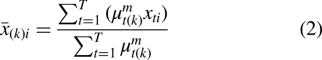 ${\bar{x}}_{(k) i} = \frac{\sum_{t = 1}^{T} (μ_{t (k)}^{m} x_{t i})}{\sum_{t = 1}^{T} μ_{t (k)}^{m}}$ (2)where $μ_{t (k)} = \frac{1}{\sum_{l = 1}^{K} {(\frac{e_{t (k)}}{e_{t (l)}})}^{\frac{2}{m - 1}}}$ (3) $e_{t (k)} = \sqrt{\sum_{i = 1}^{n} {(x_{t i} - {\bar{x}}_{(k) i})}^{2}}$ (4)where $x_{t i}$ indicates the i-th feature of example t and ${{\bar{x}}_{(k) i} | i = 1 \sim n}$ is the centroid of cluster k.

Step 3. Re-measure the distance of each example to the centroid of every cluster, and recalculate the membership.

Step 4. Stop if the following condition is satisfied. Otherwise, return to Step 2: $\underset{k}{m a x} \underset{t}{m a x} | μ_{t (k)}^{(r)} - μ_{t (k)}^{(r - 1)} | < d$ (5)where $μ_{t (k)}^{(r)}$ is the membership that example t belongs to cluster k after the r-th iteration and d is a real number representing the threshold of membership convergence.

Furthermore, to determine the optimal number of clusters (i.e. K), the separate distance test (S test) proposed by Xie and Beni⁴⁰ is applicable: $Min S$ (6)subject to $S = \frac{J_{m}}{T \cdot e_{m i n}^{2}}$ (7) $J_{m} = \sum_{k = 1}^{K} \sum_{t = 1}^{T} (μ_{t (k)}^{m} e_{t (k)}^{2})$ (8) $e_{m i n}^{2 \underset{p \neq q}{m i n} \sum_{i = 1}^{n} {({\bar{x}}_{(p) i} - {\bar{x}}_{(q) i})}^{2}}$ (9) $K \in Z^{+}$ (10)The K value that minimizes S is chosen.

Another way to determine the optimal number of clusters is through trial and error, i.e. to maximize the forecasting accuracy by varying the number of clusters.

Building prediction models

Five types of prediction models are built in the proposed methodology: DNNs (FNNs with multiple hidden layers), SVR, CART, extreme gradient boosting (XGBoost) and RFs. These methods have been widely used and are briefly introduced as follows.

DNN

DNNs are the combination of deep learning and ANNs, and there are various ways to form such combinations. In the proposed methodology, the DNN is an FNN with multiple hidden layers, as illustrated in Figure 1.

Figure 1.

Architecture of the DNN.

The inputs to the DNN are the factors related to predicting the NO_x emission of example t: { $x_{t i}$ | i = 1 ∼ n}. The inputs are propagated through the DNN as follows. First, from the input layer to the first hidden layer, the following operations are performed: $I_{t l_{1}}^{h (1)} = \sum_{i = 1}^{n} (w_{i l_{1}}^{h (1)} \cdot x_{t i})$ (11) $n_{t l_{1}}^{h (1)} = I_{t l_{1}}^{h (1)} - θ_{l_{1}}^{h (1)}$ (12) $h_{t l_{1}}^{(1)} = \frac{2}{1 + e^{- 2 n_{t l_{1}}^{h (1)}}} - 1$ (13)It is noteworthy that the transformation function is the hyperbolic tangent sigmoid function, rather than the logistic sigmoid function, that outputs a value within (−1, 1), which gives the DNN more flexibility as the output of each neuron may be negative.

Between two successive hidden layers, the following operations are performed: $I_{t l_{ξ}}^{h (ξ)} = \sum_{l_{ξ - 1} = 1}^{L_{ξ - 1}} (w_{l_{ξ - 1} l_{ξ}}^{h (ξ)} \cdot h_{t l_{ξ - 1}}^{(ξ - 1)}); ξ = 2, 3, \dots$ (14) $n_{t l_{ξ}}^{h (ξ)} = I_{t l_{ξ}}^{h (ξ)} - θ_{l_{ξ}}^{h (ξ)}; ξ = 2, 3, \dots$ 15) $h_{t l_{1}}^{(ξ)} = \frac{2}{1 + e^{- 2 n_{t l_{ξ}}^{h (ξ)}}} - 1; ξ = 2, 3, \dots$ (16)Outputs from the last hidden layer are aggregated on the output node:

$I_{t}^{o} = \sum_{l_{3} = 1}^{L_{ϑ}} (w_{l_{3}}^{o} \cdot h_{t l_{3}}^{(3)}),$ (17)and then output as $o_{t} = n_{t}^{o},$ (18)where $n_{t}^{o} = I_{t}^{o} - θ^{o} .$ (19)In equation (18), the activation (or transformation) function is the linear function. $o_{t}$ can be directly compared with actual value $y_{t}$ . With this DNN, there is no need to normalize inputs and the output. Also, the DNN may contain fewer nodes while learning faster than ANNs with a single hidden layer.⁴¹

To determine the values of network parameters, the DNN is trained using the Levenberg–Marquardt (LM) algorithm in the proposed methodology. For details refer to Suzuki.⁴²

SVR

As an extension of support vector machine (SVM), the concept of SVR is to use a kernel function to map data to a high-dimensional space to find a hyperplane and then create a decision boundary on both sides of it. If an example falls outside the boundary, the loss is calculated, as illustrated in Figure 2. Depending on the kernel function, SVM can handle linear or nonlinear problems. One advantage of SVR is that it is less prone to overfitting problems.

Figure 2.

The concept of SVR.

SVR aims to fit a multiple regression function to predict the output according to the inputs. The multiple regression function can be written as: $o_{t} = \sum_{i = 1}^{n} w_{i} ϕ (x_{t i}) + b .$ (20)where $ϕ ()$ is the kernel function. The value of $w_{i}$ can be derived by solving the following optimization problem: $Min R = \frac{1}{2} w^{T} w + C \sum_{t = 1}^{T} (ξ_{t} + {\hat{ξ}}_{t}) .$ (21)subject to $o_{t} - y_{t} \leq ε + ξ_{t}; t = 1 \sim T$ (22) $y_{t} - o_{t} \leq ε + {\hat{ξ}}_{t}; t = 1 \sim T$ (23) $ξ_{t}, {\hat{ξ}}_{t} \geq 0; t = 1 \sim T$ (24)where ε is the distance between the two decision boundaries. $ξ_{t}$ (or ${\hat{ξ}}_{t}$ ) is the distance of example t to the decision boundary if it falls outside the boundary.

CART

The procedure for constructing a CART is composed of three stages: tree growing, stopping and pruning. The first stage is growing a tree using a recursive partitioning technique that selects a variable and a split point according to the prespecified criterion. Common criteria include Gini, towing, ordered towing and maximum-deviance reduction.⁴³ This study adopts the last criterion.

Let $Ω_{m}$ be the set of examples belonging to node m that is to be split into two branches with sets $Ω_{m}^{L}$ and $Ω_{m}^{R}$ ; m = 1 ∼ M. For either set, the predicted NO_x emissions of all examples are averaged as the predicted value: $o_{m}^{L / R} = \frac{\sum_{t \in Ω_{m}^{L / R}} o_{t}}{| Ω_{m}^{L / R} |}$ (25)The split that minimizes the sum of squared error (SSE) is chosen: $S S E = \sum_{m = 1}^{M} \sum_{t \in Ω_{m}} (y_{t} - o_{m})^{2}$ (26)Starting from the largest tree, the CART is pruned until the following objective function is minimized: $Min C = \sqrt{\frac{S S E}{M}} + α | S |$ (27)where $| S |$ indicates the size of the CART (in terms of the number of nodes or branches) and α is a positive constant.

XGBoost

XGBoost is a popular machine learning algorithm in recent years. The algorithm was proposed by Chen and Guestrin.⁴⁴ It is an extension of gradient boosting decision tree (GBDT) that combines the advantages of bagging and boosting. The former performs feature sampling in a random manner; the latter generates trees in a sequential manner. A tree generated later is related to the previous tree and can correct the error of the latter.

RF

A RF consists of multiple decision trees, each of which is constructed based on a replaceable sampling of the training data, that is, bootstrapping. Due to replacement after random sampling, some data may be double-selected and some will never be selected. The latter is called out-of-bag (OOB) data. Random samples are used to build/train a forest of multiple decision trees to predict the NO_x emission. The trained decision trees are then applied to make predictions for the OOB data. The predictions produced by all decision trees are averaged; on this basis, the prediction performance is evaluated in terms of RMSE: $RMSE = \sqrt{\frac{1}{T} \sum_{t = 1}^{T} {(o_{t} - y_{t})}^{2}}$ (28)

Aggregation

An example can be classified into multiple clusters to various degrees using FCM. Therefore, the prediction models of these clusters can be applied to make predictions for the example. Then, these prediction results are aggregated. To this end, three aggregators are considered: FNN,^45,46 SVR and RF, as illustrated in Figure 3. Inputs to these aggregators are the memberships of the example to various clusters and the corresponding prediction results. Among possible aggregators, the most accurate one that minimizes RMSE will be chosen. The output from the aggregator, the aggregation result, is the predicted NO_x emission.

Figure 3.

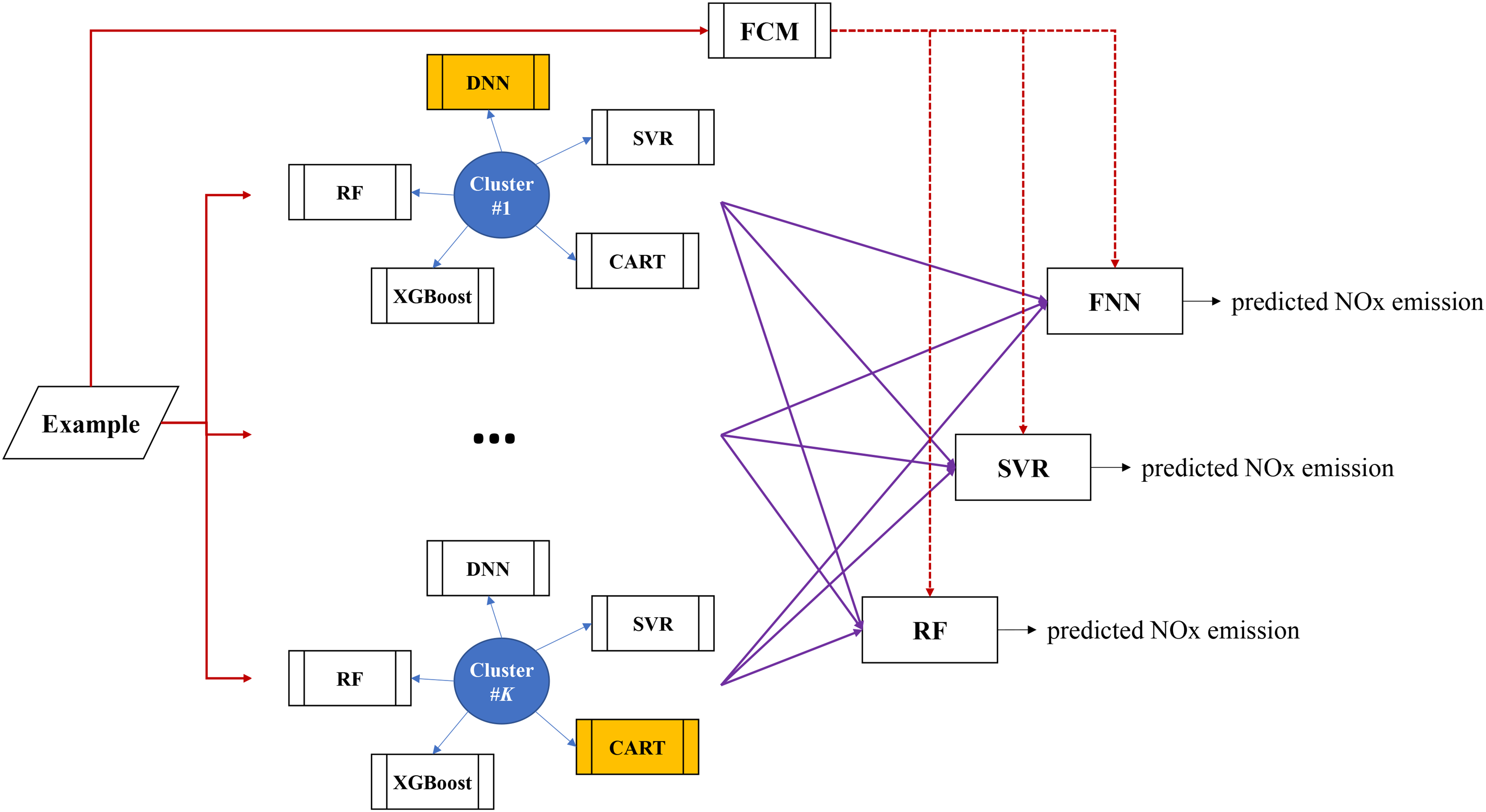
The aggregation process.

Case study

Background

To illustrate the applicability of the proposed methodology, it has been applied to analyze the coal combustion-related data provided by a thermal power plant in Taiwan. In the proposed methodology, XGBoost, SVR, RF and decision trees were implemented using Python, which selected hyperparameters using grid search to facilitate model optimization. FCM and FNNs (or DNNs) were constructed using the related toolboxes of MATLAB.

The data collection period was from January 2019 to December 2019. The collected data included 317 examples (i.e. coal batches). Input variables to each prediction model were the specification and composition of coal in terms of 19 features: heating value (as received), heating value (air dried), ash, sulphur, volatile nitrogen, coke nitrogen, total moisture, inherent moisture, grinding rate, Na₂O, CaO, MgO, Fe₂O₃, K₂O, SiO₂, Al₂O₃, TiO₂, softening point and air. The output from the prediction model was the NO_x emission (ppm).

Application of the proposed methodology

First, box-and-whisker plots were used to identify outliers, that is, values that fell outside 1.5 times the interquartile range of Q1 and Q3, to remove them. As a result, the number of examples reduced to 243.

Then, feature selection was carried out using RF-RFE with cross-validation. The importance of features evaluated by RF were ranked. The result is presented in Table 2. In the subsequent process of combustion, volatile nitrogen and coke nitrogen are burned to generate NO_x and N2 respectively, so the final products of fuel nitrogen after complete combustion are NO_x and nitrogen. After removing the least important features, the model was re-trained. Finally, the best number of features was determined as 15. CV was set to 3. Therefore, input variables to each prediction model included heating value (as received), ash, sulphur, volatile nitrogen, coke nitrogen, inherent moisture, grinding rate, Na₂O, CaO, MgO, Fe₂O₃, K₂O, SiO₂, softening point and air. The prediction accuracy, in terms of mean absolute percentage error (MAPE) and RMSE, using various prediction models before and after feature selection is compared in Table 3. After feature selection, the prediction accuracy of most forecasting models was improved.

Table 2.

Ranking the importance of features.

Rank	Feature	Importance
1	Volatile nitrogen	0.1241
2	Air	0.0997
3	Inherent moisture	0.0808
4	Sulphur	0.0707
5	Coke nitrogen	0.0695
6	Softening point	0.0616
7	Grinding rate	0.0491
8	Fe₂O₃	0.0475
9	K₂O	0.0459
10	Heating value (as received)	0.0457
11	CaO	0.0435
12	SiO₂	0.0412
13	Ash	0.0398
14	Na₂O	0.0366
15	MgO	0.0340
16	Heating value (dry)	0.0329
17	Al₂O₃	0.0286
18	Total moisture	0.0248
19	TiO₂	0.0238

Table 3.

Comparison of prediction performances using various models before and after feature selection.

Prediction model	Hyperparameters	MAPE (Before feature selection)	MAPE (After feature selection)	RMSE (ppm) (Before feature selection)	RMSE (ppm) (After feature selection)
XGBoost	Learning rate = 0.005 Maximum depth = 2 Number of estimators = 1500	10.4%	9.6%	16.15	15.65
SVR	Kernel function: radial basis function (RBF) C = 20 Gamma = 0.5	11.6%	10.9%	19.30	18.6
RF	Maximum depth = 6 Number of estimators = 100	10.6%	10.0%	17.58	15.96
Decision tree	Maximum depth = 3 Minimum samples per leaf = 3 Minimum samples per split = 4	12.0%	12.8%	19.5	20.17
DNN	Training function = Bayesian regularization Number of hidden layers = 2	12.8%	10.7%	17.92	17.72

Subsequently, the collected data were divided into two and three clusters using FCM, and the most suitable model for each cluster was identified. Then, the data of each cluster were randomly divided into 60% for training the prediction model (XGBoost, SVR, RF, decision tree or DNN), 30% for training the aggregation model (FNN, SVR or RF) and 10% for evaluating the prediction performance. The hyperparameters of XGBoost, SVR, RF and decision trees were optimized using grid search by setting CV to 3, as shown in Table 4. In addition, the number of hidden layers in the DNN and the number of neurons in each hidden layer were selected by trial and error. Each configuration of the DNN was trained 10 times, and the optimal configuration was determined based on the average performance.

Table 4.

Hyperparameters of various prediction models.

Prediction model	Hyperparameters	Possible values
XGBoost	Learning rate Maximum depth Number of estimators	(0.001, 0.005, 0.01, 0.1) (2, 3, 4, 7, 9) (100, 200, 500, 1000, 1200, 1500)
SVR	Kernel function C Gamma	(Polynomial, rbf, sigmoid) (0.01, 0.1, 0.3, 0.5, 0.8, 1, 3, 10, 15, 20) (0.001, 0.005, 0.01, 0.05, 0.1, 0.5)
RF	Maximum depth Number of estimators	(5–9) (50, 100, 300, 500)
Decision tree	Maximum depth Minimum samples per leaf Minimum samples per split	(3, 5, 7, 9, 11, 20, 30, 50) (1–5) (1–5)
DNN	Training function Number of hidden layers Number of nodes in each hidden layer	(Bayesian regularization, Levenberg–Marquardt) (1–2) (1–15)

First, the collected data were divided into two clusters. By assigning each example to the cluster with the highest membership, the first cluster had 70 examples, and the second cluster had 75 examples. Then, a suitable prediction model was constructed for each cluster. After comparison, DNN and SVR were suitable for the two clusters in predicting the NO_x emission, as shown in Table 5. Subsequently, the collected data were divided into three clusters. The prediction models suitable for the three clusters are summarized in Table 6.

Table 5.

Suitable prediction model for each cluster (two clusters).

Cluster No.	Suitable prediction model	Hyperparameters	MAPE	RMSE (ppm)
1	DNN	Training function: Bayesian regularization Two hidden layers with one and three nodes	10.2%	15.26
2	SVR	Kernel function: rbf C: 20 Gamma: 0.5	10.2%	14.42

Table 6.

Suitable prediction model for each cluster (three clusters).

Cluster No.	Suitable prediction model	Hyperparameters	MAPE	RMSE (ppm)
1	DNN	Training function: Levenberg–Marquardt Two hidden layers with 13 and 1 nodes	7.4%	10.86
2	DNN	Training function: Levenberg–Marquardt Two hidden layers with 14 and 1 nodes	8.1%	12.72
3	SVR	Kernel function: rbf C: 20 Gamma: 0.5	9.2%	15.10

When a new example came in, the prediction models of all clusters were applied to make predictions, since it was not possible to absolutely classify the example to a single cluster. Then, all prediction results were aggregated. The predicted value by the prediction model of each cluster and the membership that the example belonged to the cluster were used as inputs to the aggregation model.^47,48 The output was the predicted NO_x emission. The prediction performances using various aggregators were compared. According to the comparison results, RF and SVR were the most suitable aggregators, respectively, when there were two and three clusters, as shown in Table 7. In contrast, without data clustering, the prediction accuracy was MAE = 10.7% and RMSE = 17.72 (ppm). Obviously, dividing the collected into three clusters helped improve the prediction performance.

Table 7.

Prediction performance after aggregation.

Number of clusters	Suitable aggregation model	Hyperparameters	MAPE	RMSE (ppm)
2	RF	Maximum depth: 5 Number of estimators: 300	13.8%	19.05
3	SVR	Kernel function: rbf C: 20 Gamma: 0.001	9.0%	14.55

Discussion

According to the experimental results, the following discussion was carried out:

From Table 7, it can be easily seen that after feature selection, dividing the collected data into three clusters and then aggregating the prediction results of all clusters with SVR achieved quite good prediction performance. MAPE was only 8.9%, while RMSE also dropped to 14.55 ppm. However, if the collected data were divided into only two clusters, the improvement in the prediction performance was not significant.

The effects of different input variables on the output value were not equal. In addition, such effects varied across different prediction models. Table 8 lists the top three input variables that have the most significant effects on the predicted NO_x emission in different prediction models. It can be found that volatile nitrogen, air and grinding rate had the top three effects on the predicted NO_x emission in most prediction models, so the three factors can be adjusted if the predicted NO_x emission is to be reduced, as shown in Table 9. Using most prediction models, the predicted NO_x emission increases when volatile nitrogen decreases or grinding rate increases. In addition, when air decreases, the NO_x emission drops as well.

Table 8.

Top three input variables with the most significant effects on the predicted NO_x emission in various prediction models.

Prediction model	Top three input variables
XGBoost	Air, volatile nitrogen and grinding rate
SVR	Air, volatile nitrogen and softening point
RF	Air, grinding rate and volatile nitrogen
Decision tree	Volatile nitrogen and air softening point
DNN	Volatile nitrogen, coke nitrogen and grinding rate

Table 9.

Adjusting three input variables to reduce the predicted NO_x emission.

Predicted NO_x emission	Air		Volatile nitrogen		Grinding rate
Predicted NO_x emission	+10%	−10%	+10%	−10%	+10%	−10%
XGBoost	+1.19%	−6.00%	−2.52%	+3.79%	+0.19%	+4.14%
SVR	+5.25%	−5.95%	−4.23%	+5.34%	+2.06%	−1.22%
RF	+1.18%	−2.67%	−1.80%	+4.27%	+4.03%	−0.60%
Decision tree	−1.28%	−1.62%	−1.04%	+12.93%	+0.00%	−0.00%
DNN	+7.70%	−6.39%	−7.20%	+12.27%	+10.05%	−6.80%

Comparison with existing methods

To further elaborate the effectiveness of the proposed methodology, 10 existing methods have also been applied to the collected data for comparison: LSTM,¹⁹ XGBoost,⁴⁹ RFECV + XGBoost, SVR, RFECV + SVR, RF,⁴⁹ RFECV + RF, decision trees,⁴⁹ RFECV + decision trees, DNN and RFECV + DNN.⁵⁰ In the LSTM method, the learning rate varied from 0.005 to 0.05 and the selection of the timestep was set to 5. The forecasting accuracy, in terms of MAPE and RMSE, using various methods is summarized in Table 10. Obviously:

The proposed methodology achieved a better forecasting accuracy by minimizing MAPE and RMSE. The advantage over existing methods was up to 30% in reducing MAPE.

Feature selection using RFECV was conducive to the prediction performances of most existing methods except decision trees. The effect was most significant when RFECV was applied to DNN.

Compared with the benchmark study by Yang et al.,¹⁹ the predictive performance using the LSTM method was worse when coal composition is considered instead of combustion parameters and conditions. However, as a pretreatment, coal screening by composition remains an interesting attempt, as this has added value for optimizing subsequent combustion processes.

Table 10.

Prediction accuracy using various methods.

Method	MAPE	RMSE (ppm)
LSTM¹⁹	9.2%	15.50
XGBoost⁴⁹	10.4%	16.15
RFECV + XGBoost	9.6%	15.65
SVR	11.6%	19.30
RFECV + SVR	10.9%	18.60
RF⁴⁹	10.6%	17.58
RFECV + RF	10.0%	15.96
Decision trees⁴⁹	12.0%	19.50
RFECV + decision trees	12.8%	20.17
DNN	12.9%	17.92
RFECV + DNN⁵⁰	10.7%	17.72
Proposed methodology	9.0%	14.55

Conclusions

With the rise of environmental awareness, more and more people are paying attention to the impact of air quality on health. As one of the main sources of air pollution, thermal power generation has attracted much attention. Governments around the world are also targeting the pollutants emitted by thermal power plants. A series of preventive measures have been taken to prevent pollution, including installing high-efficiency electrostatic precipitators to reduce the escape of fine aerosols, installing flue gas desulfurization equipment to reduce the production of SO₂ and building low-NO_x burners and SCR equipment for NO_x.

The proportion of NO_x in the pollutants of coal-fired units is the largest. Therefore, the accurate prediction of NO_x emissions after coal combustion is very important for the prevention and control of air pollution. For this purpose, from a novel perspective, this study proposes a fuzzy big data analytics approach, which takes the coal composition as input, and predicts the NO_x emission level after coal combustion using fuzzy big data analytics techniques such as feature selection, fuzzy clustering and fuzzy aggregation. The contribution of this study is the selection of better coal for combustion to reduce NO_x emissions, in addition to ex post pollution reduction strategies. It provides a new approach for thermal power plants to reduce NO_x emissions.

The effectiveness of the fuzzy big data analytics approach has been examined using a real case study. According to experimental results:

If the data were not clustered, XGBoost and RF achieved the best prediction performances. Their MAPEs were only 9.6% and 10.04%, respectively.

Feature selection has improved the prediction performances of most existing prediction models.

Clustering the collected data into three clusters also improved the prediction accuracy.

After clustering the collected data into three clusters, SVR and DNN were the most suitable prediction models for these clusters in optimizing the prediction accuracy.

SVR was shown to be the most effective method in aggregating the prediction results of all clusters.

In future studies, different clustering methods such as mean-shift algorithm, Gaussian mixture model, density based spatial clustering algorithm with noise and density peak clustering can be applied to compare their results. In addition, PCA can be applied in data preprocessing to project high-dimensional data into a low-dimensional space through linear transformation, which can reduce the complexity and remove noise.

Contributorship

All authors contributed equally to the writing of this paper.

Footnotes

Declaration of conflicting interests

The author(s) declared no potential conflicts of interest with respect to the research,authorship,and/or publication of this article.

Funding

The author(s) received no financial support for the research,authorship,and/or publication of this article.

ORCID iDs

Tin-Chih Toly Chen

Yu-Cheng Wang

References

Wendt

JOL

. Fundamental coal combustion mechanisms and pollutant formation in furnaces. Prog Energy Combust Sci 1980; 6: 201–222.

Agarwal

Mangal

Satsangi

, et al. Characterization, sources and health risk analysis of PM2.5 bound metals during foggy and non-foggy days in sub-urban atmosphere of Agra. Atmos Res 2017; 197: 121–131.

Abdolahnejad

Jafari

Mohammadi

, et al. Cardiovascular, respiratory, and total mortality ascribed to PM10 and PM2.5 exposure in Isfahan, Iran. J Educ Health Promot 2017; 6: 09.

Chen

de la Campa

AMS

, et al. 2005–2014 Trends of PM10 source contributions in an industrialized area of southern Spain. Environ Pollut 2018; 236: 570–579.

World Health Organization. Health effects of particulate matter: policy implications for countries in eastern Europe, Caucasus and central Asia, https://apps.who.int/iris/bitstream/handle/10665/344854/9789289000017-eng.pdf?sequence=1 (2013).

Greenberg

Carel

Derazne

, et al. Different effects of long-term exposures to SO₂ and NO₂ air pollutants on asthma severity in young adults. J Toxicol Environ Health, Part A 2016; 79: 342–351.

Gimeno

Marı´n

Del Teso

, et al.

How effective has been the reduction of SO₂ emissions on the effect of acid rain on ecosystems?

Sci Total Environ 2001; 275: 63–70.

Anderson

Hawkins

Jones

. CO₂, the greenhouse effect and global warming: from the pioneering work of Arrhenius and Callendar to today’s Earth System Models. Endeavour 2016; 40: 178–187.

Chauhan

Krishna

Frew

, et al. Exposure to nitrogen dioxide (NO₂) and respiratory disease risk. Rev Environ Health 1998; 13: 73–90.

10.

Thurston

. Outdoor air pollution: sources, atmospheric transport, and human health effects. Int Encycl Public Health 2008; 2008: 700–712.

11.

Zhong

Yuan

, et al. The feasibility of clean power generation from a novel dual-vertical-well enhanced geothermal system (EGS): a case study in the Gonghe Basin, China. J Cleaner Prod 2022; 344: 131109.

12.

Cui

Liao

, et al. A short-term hybrid energy system robust optimization model for regional electric-power capacity development planning under different pollutant control pressures. Sustainability 2021; 13: 11341.

13.

Dong

Jiang

, et al. Life cycle assessment of coal-fired solar-assisted carbon capture power generation system integrated with organic Rankine cycle. J Cleaner Prod 2022; 356: 131888.

14.

Shi

. The COVID-19 pandemic and energy transitions: evidence from low-carbon power generation in China. J Cleaner Prod 2022; 368: 132994.

15.

Belosevic

Beljanski

Tomanovic

, et al. Numerical analysis of NO x control by combustion modifications in pulverized coal utility boiler. Energy Fuels 2012; 26: 425–442.

16.

Diez

Cortés

Pallarés

. Numerical investigation of NO_x emissions from a tangentially-fired utility boiler under conventional and overfire air operation. Fuel 2008; 87: 1259–1269.

17.

Hill

Smoot

. Modeling of nitrogen oxides formation and destruction in combustion systems. Prog Energy Combust Sci 2000; 26: 417–458.

18.

H-C

Chen

T-CT

Chiu

M-C

. Constructing a precise fuzzy feedforward neural network using an independent fuzzification approach. Axioms 2021; 10: 282.

19.

Yang

Wang

. Prediction of the NO_x emissions from thermal power plant using long-short term memory neural network. Energy 2020; 192: 116597.

20.

Yuan

Meng

Bai

Cui

Jiang

(2021). Prediction of NOx emissions for coal-fired power plants with stackgeneralization ensemble method. Fuel, 289, 119748.

21.

Wang

Liu

Wang

, et al. A hybrid NO_x emission prediction model based on CEEMDAN and AM-LSTM. Fuel 2022; 310: 122486.

22.

Al-Refaie

Judeh

Chen

. Optimal multiple-period scheduling and sequencing of operating room and intensive care unit. Operat Res 2018; 18: 645–670.

23.

Chen

T-CT

. Type-II fuzzy collaborative intelligence for assessing cloud manufacturing technology applications. Robot Comput Integr Manuf 2022; 78: 102399.

24.

Lin

Chen

. A ubiquitous clinic recommendation system using the modified mixed-binary nonlinear programming-feedforward neural network approach. J Theor Appl Electron Commer Res 2021; 16: 3282–3298.

25.

Wang

Chen

TCT

. Assessing and comparing COVID-19 intervention strategies using a varying partial consensus fuzzy collaborative intelligence approach. Mathematics 2020; 8: 1725.

26.

Chang

. Predicting NO_x emissions from coal combustion composition-using a fuzzy-neural clustering prediction method. Master Thesis, National Yang Ming Chiao Tung University, 2022.

27.

Quérel

Grondin

Letellier

. State of the art and analysis of control oriented NO_x models. SAE Technical Paper 2012-01-0723, 1–17, 2012.

28.

Van Der Lans

Glarborg

Dam-Johansen

. Influence of process parameters on nitrogen oxide formation in pulverized coal burners. Prog Energy Combust Sci 1997; 23: 349–377.

29.

Nazari

Shahhoseini

Sohrabi-Kashani

, et al. Experimental determination and analysis of CO₂, SO₂ and NO_x emission factors in Iran’s thermal power plants. Energy 2010; 35: 2992–2998.

30.

Cobourn

Bai

. Development of nonlinear empirical models to forecast daily PM2.5 and ozone levels in three large Chinese cities. Atmos Environ 2016; 147: 209–223.

31.

Smrekar

Pandit

Fast

, et al. Prediction of power output of a coal-fired power plant by artificial neural network. Neural Comput Appl 2010; 19: 725–740.

32.

Madhavan

K. S.

Reddy

T. K.

Krishnaiah

Dhanuskodi

Sowmiya

. (2012). Development of artificial neural network (ANN) based prediction model for NOx emissions from utility boilers. In Proceedings of the International Conference on Advanced Research in Mechanical Engineering, pp. 1–3.

33.

Zhou

Zhao

J. P.

Zheng

L. G.

Wang

C. L.

Cen

K. F

. (2012). Modeling NOx emissions from coal-fired utility boilers using support vector regression with ant colony optimization. Engineering Applications of Artificial Intelligence, 25(1), 147–158.

34.

Yang

Liu

Wang

Ding

Huang

. (2019). Reaction mechanism for NH3-SCR of NOx over CuMn2O4 catalyst. Chemical engineering journal, 361, 578–587.

35.

Chen

. (2011). Applying a fuzzy and neural approach for forecasting the foreign exchange rate. International Journal of Fuzzy System Applications, 1(1), 36–48.

36.

H. C.

Chen

. (2015). CART–BPN approach for estimating cycle time in wafer fabrication. Journal of Ambient Intelligence and Humanized Computing, 6, 57–67.

37.

Al-Refaie

Chen

Al-Athamneh

, et al. Fuzzy neural network approach to optimizing process performance by using multiple responses. J Ambient Intell Humaniz Comput 2016; 7: 801–816.

38.

Chen

Wang

. Incorporating the FCM–BPN approach with nonlinear programming for internal due date assignment in a wafer fabrication plant. Robot Comput Integr Manuf 2010; 26: 83–91.

39.

Chen

T. C. T.

Honda

. (2020). Introduction to fuzzy collaborative forecasting systems. Fuzzy Collaborative Forecasting and Clustering: Methodology, System Architecture, and Applications, 1–8.

40.

Xie

X. L.

Beni

. (1991). A validity measure for fuzzy clustering. IEEE Transactions on Pattern Analysis & Machine Intelligence, 13(08), 841–847.

41.

Wang

Chen

Hsu

. A fuzzy deep predictive analytics approach for enhancing cycle time range estimation precision in wafer fabrication. Decis Anal J 2021; 1: 100010.

42.

Suzuki

Ochiai

Mitsuda

Imai

Manabe

, Kikuchi, K., … & Shiotani, M. (2011, July). Verification of pointing and antenna pattern knowledge of Superconducting Submillimeter-Wave Limb-Emission Sounder (SMILES). In 2011 IEEE International Geoscience and Remote Sensing Symposium, pp. 3688–3691.

43.

Loh

. Classification and regression trees. Wiley Interdiscip Rev Data Min Knowl Discov 2011; 1: 14–23.

44.

Chen

Guestrin

. Xgboost: a scalable tree boosting system. Proceedings of the 22nd ACM SIGKDD International Conference on Knowledge Discovery and Data Mining, 2016, pp. 785–794.

45.

Chen

Wang

. Estimating simulation workload in cloud manufacturing using a classifying artificial neural network ensemble approach. Robot Comput Integr Manuf 2016; 38: 42–51.

46.

Lin

Wang

Chen

TCT

, et al. Evaluating the suitability of a smart technology application for fall detection using a fuzzy collaborative intelligence approach. Mathematics 2019; 7: 1097.

47.

Lin

Chen

TCT

. Leisure agricultural park selection for traveler groups amid the COVID-19 pandemic. Agriculture 2022; 12: 111.

48.

Chiu

M-C

Chen

. Assessing mobile and smart technology applications to active and healthy ageing using a fuzzy collaborative intelligence approach. Cognit Comput 2021; 13: 431–446.

49.

Yim

SHL

. High temporal resolution prediction of street-level PM2.5 and NO_x concentrations using machine learning approach. J Cleaner Prod 2020; 268: 121975.

50.

Shin

Lee

Park

, et al. Predicting transient diesel engine NO_x emissions using time-series data preprocessing with deep-learning models. Proc Inst Mech Eng D: J Automob Eng 2021; 235: 3170–3184.

Improving people's health by burning low-pollution coal to improve air quality for thermal power generation

Abstract

Keywords

Introduction

Literature review

Methodology

Procedure

Feature selection

Data clustering

Building prediction models

DNN

SVR

CART

XGBoost

RF

Aggregation

Case study

Background

Application of the proposed methodology

Discussion

Comparison with existing methods

Conclusions

Contributorship

Footnotes

Declaration of conflicting interests

Funding

ORCID iDs

References