A Practical Guide to Specifying Random Effects in Longitudinal Dyadic Multilevel Modeling

Abstract

Analyzing over-time dyadic data can be challenging, particularly when using multilevel models with complex random-effect structures. In this tutorial, we discuss the best practices of model specification for longitudinal dyadic multilevel modeling, providing a practical guide to specifying (and respecifying) random effects with both theoretical and practical considerations in mind. We begin by defining random effects in the context of repeated-measures dyadic data and address common issues such as nonconvergence. Then, using two models—the dyadic growth-curve and the stability and influence model—we demonstrate how to apply these guidelines in both SAS and R. The dyadic growth-curve model provides a straightforward example, whereas the stability and influence model illustrates common challenges when dealing with complex random-effect structures and convergence issues. In the first exercise, we explain how to customize the variance-covariance matrix for these analyses in SAS. In the second exercise, we adapt these analyses for R and discuss how to implement the sum-and-difference approach for indistinguishable dyads. We conclude with a discussion of alternative models and go over the utility of data simulation during study design, helping readers plan and select the best approach for their research.

Relationship scholars have long been interested in studying how relationship processes develop over time, ranging from gradual processes, such as how couples converge in their personality traits (Oltmanns et al., 2020), emotional responses (Anderson et al., 2003), and sleep patterns (Gordon et al., 2021; Gunn & Eberhardt, 2019), to more immediate changes, such as when partners converge in their physiologic states (Davidesco et al., 2023; del Rosario et al., 2024, 2025; West & Mendes, 2023; Wohltjen et al., 2023), linguistic patterns of speech (Templeton et al., 2022, 2023), and nonverbal behaviors (e.g., Mayo & Gordon, 2020) within a single conversation.

Studying over-time processes in dyads requires balancing theoretical questions (Do I care about modeling the covariances between two partners’ slopes, which captures whether their rates of change are similar?) with practical considerations (Will the model converge if I model the covariances between slopes?). Although there are plenty of resources on multilevel modeling (MLM) and dyadic analysis (for a review, see Gordon & Thorson, 2024; Kashy & Kenny, 2000), in this tutorial, we focus specifically on one component of the model that poses both conceptual and practical challenges: the random effects. We focus on why they matter, how to specify them across different statistical programs, and how to manage nonconvergence issues.

Random effects are important because they capture the natural variability between individuals or dyads without needing to identify why those differences exist (Bolger & Laurenceau, 2013). If there are sources of nonindependence in the data, such as individuals nested within couples or repeated measures within persons—as is often the case in longitudinal dyadic data—failing to account for random effects can result in misspecified models and overlook theoretically meaningful interpersonal processes. This tutorial is designed for researchers interested in analyzing over-time dyadic data and provides guidelines that address important theoretical and practical considerations, starting with the proper conceptualization of random effects.

Examples of Longitudinal Dyadic Models

The issues we discuss apply broadly to dyadic MLM with repeated-measures data. Here, we focus on two for illustration: the dyadic growth-curve model and the stability and influence model. The dyadic growth-curve model tracks change over time for both members of a dyad, in which the interest is in modeling the strength of that over-time change (Raudenbush et al., 1995; Rogers et al., 2018). For example, one might model changes in relationship satisfaction over the first year of marriage in a study among newlyweds, assuming that there is variability in rates of change (e.g., some people increase and some decrease in satisfaction). The dyadic growth-curve model is typically more straightforward and introduces fewer complications than our second model: the stability and influence model.

The stability and influence model is an extension of the cross-lagged panel model (CLPM) and uses a multilevel framework to evaluate (a) the degree to which one partner’s score on an outcome measure at one time point predicts the other partner’s score at a future time point (e.g., Brown et al., 2021; Helm et al., 2014; Liu et al., 2013; K. R. Thorson et al., 2018; West & Mendes, 2023) and (b) the degree to which each partner is stable from one moment to the next in the outcome measure. In other words, the “influence” component of this model refers to the cross-lagged effect, and “stability” describes the autoregressive effect. For instance, in a daily diary study, one might explore how a husband’s stress predicts his wife’s stress at the next time point (influence) while accounting for how stable both partners’ stress levels are from day to day (stability). Another conceptually related model is the longitudinal actor–partner interdependence model (L-APIM), which, just like the stability and influence model, applies the logic of the CLPM to dyads by modeling both autoregressive and cross-lagged effects and typically examines how one variable predicts a different outcome in a partner (e.g., whether depression predicts changes in a partner’s relationship satisfaction).

We focus on the dyadic growth-curve model and the stability and influence model for several reasons. First, these models are versatile and can be used with a wide range of measures (e.g., behavioral, physiologic, linguistic), making them popular tools for studying dynamic processes across contexts, including naturalistic conversations (del Rosario et al., 2025; Kraus & Mendes, 2014; Ryjova et al., 2024), relationship outcomes (Gander et al., 2025; Olson et al., 2023), learning interactions (Davidesco et al., 2023; K. R. Thorson et al., 2019), and interactions in the field (del Rosario et al., 2024; Gordon et al., 2022). Second, these models allow for the inclusion of moderators (e.g., in the stability and influence model, one can test whether the direction and strength of influence vary by the social status of the person doing the influencing and the person being influenced; K. R. Thorson et al., 2021). Third, because these are dyadic multilevel models, there are several random effects that can be estimated, including covariances within persons (If an individual is stable, is the individual more or less influenced?) and between dyad members (If an individual is stable, is the individual partner also stable?). Finally, convergence problems are common, and there is little guidance to date on how to handle them. Thus, in this tutorial, we cover a systematic approach to respecifying the model to achieve convergence.

There is an ongoing debate about the merits of the CLPM (and autoregressive models more generally) and its appropriateness for different types of data (see Lucas, 2023). Critics have argued that the CLPM conflates within-persons change with between-persons trait differences and, in turn, potentially inflates cross-lagged effects (Andersen, 2022; Hamaker et al., 2015). The random-intercept cross-lagged panel model (RI-CLPM) addresses this issue by modeling random intercepts as latent variables, essentially subtracting out trait-level differences. What remains in the autoregressive and cross-lagged paths are pure within-units change. The CLPM, on the other hand, does not separate trait-level variability from within-persons fluctuations. It assumes that all individuals (or dyads) vary around the same group mean and that no one has a stable “set point” that carries across all time points, conflating trait differences and influence (Hamaker et al., 2015; Lucas, 2023).

The decision between CLPM and RI-CLPM depends on both the conceptual question and features of the data. Starting with conceptual differences, the RI-CLPM subtracts out trait differences, treating trait as a nuisance rather than a point of interest in the data. This model is particularly useful if the interest is in modeling within-persons change (e.g., “When a child is more depressed than usual, does the parent also feel more depressed later on?”), whereas the CLPM can answer questions about between-persons effects (e.g., “Do children with higher average depression also tend to have parents with higher average depression?”) and how trajectories differ across people (e.g., “Does a child’s change in depression relate to the parent’s change in depression?”; Orth et al., 2021).

The time between measurements is also important to consider. For many panel studies in psychology, measurements (or waves) might be weeks, months, or even years apart. When waves are too spread out to capture psychological change, the CLPM cross-lags pick up on trait correlations leading to spurious effects (Dormann & Griffin, 2015) or effects that contradict theory (Swider & Zimmerman, 2014). Shorter intervals between measurements can minimize the chances of false positives in the cross-lagged effects. Dormann and Griffin (2015) recommended shorter time lags because they account for bias in the stability path. Many psychological processes are small and may be difficult to capture if the lag between measurements is too long or infrequent. In high-frequency data (e.g., interbeat intervals [IBIs]; i.e., time-based measure representing the milliseconds between heartbeats, posture or facial expressions measured in 30-s intervals, or vocal tone throughout a conversation), the underlying “trait” hardly changes from moment to moment. If one were to sample IBIs, which are measured continuously, the last interval will not be wildly different from the next—the change is gradual. Unlike other multiwave data, the stability path for high-frequency data, such as physiology, tends to be very high (K. R. Thorson et al., 2018). Therefore, it is unlikely that the cross-lagged effects are driven by spurious effects. In fact, if there were large changes between successive measurements, they would be flagged as physiologically implausible and treated as an artifact in the data. Given that the data we use to illustrate the stability and influence model are measured continuously (averaged in 30-s bins), fluctuations are going to be incremental, so the cross-lagged effects are not likely an artifact of trait drift. However, we assume that researchers are at the analysis stage after theoretical justification has been made and the criticisms of this approach made by others (Berry & Willoughby, 2017; Hamaker et al., 2015; Lucas, 2023) have been considered.

We begin this tutorial with a theoretical foundation, explaining what random effects are in the context of repeated-measures dyadic data. We compare two common frameworks for analyzing over-time dyadic data: MLM and structural equation modeling (SEM). We then shift the focus to MLM and address common issues, including nonconvergence—why it happens, how to design studies that maximize the likelihood of finding random variance, and strategies for troubleshooting when convergence issues arise. We demonstrate model specification in two parts. First, we walk through how to customize the variance-covariance matrix for random effects, which we refer to as the “G matrix” (Fiedler & Hall, 2012) in SAS. Then, we show how to adapt this code for R by using predefined random matrices for distinguishable dyads and the sum-and-difference method for indistinguishable dyads. We focus on developing an understanding of random variances and covariances to prevent an overreliance on any single model, especially when trimming random effects might be necessary. In each exercise, we first demonstrate these concepts using the dyadic growth-curve model and then explain how they apply to the more complex stability and influence model. Finally, we discuss alternative models and offer recommendations, including guidance on using data simulations to help with model selection during study design. All materials, including the data and code for both SAS and R, are available on OSF (https://osf.io/yf9gq/?view_only=d079fb9d36aa444b88b2e8ed2144ec3a).

Understanding Random Effects in Dyadic Repeated-Measures Models

Random effects are the unsung heroes of longitudinal dyadic analysis. They not only account for sources of nonindependence (e.g., correlations between multiple responses within an individual and between dyad members), but they can also reveal meaningful heterogeneity in the data (Bolger et al., 2019). Fixed and random effects are two sides of the same coin. Fixed effects estimate average patterns across people, and random effects capture how much those patterns vary. Suppose one wants to model couples’ stress during the first year of marriage. A fixed intercept represents the expected value of an outcome when all predictors are set to zero. If time is included as a predictor, “Day 0” may not exist in the data. So, one centers time such that Day 0 represents the first day of the study. Now, the fixed intercept can be interpreted as the average stress at the start of the study, and the random intercept represents how much couples vary in their baseline stress levels. A random slope for time is included to capture whether people differ in how their stress levels change over time. The within-persons covariance between the random intercept and slope tells whether individuals’ baseline levels of stress are related to how their stress levels change over time (e.g., Do people who start off lower in stress tend to show a steeper increase in stress?). In dyadic models, one can go a step further by modeling how partners’ variability in responses relate to one another. These include between-persons intercept covariances (e.g., Are individuals’ baseline stress levels associated with their partners’ baseline stress levels?), between-persons slope covariances (e.g., Are partners’ changes in stress over time related?), and between-persons intercept-slope covariances (e.g., Is one person’s baseline stress related to how the person’s partner’s stress changes over time?). These types of questions illustrate how random effects can help one understand patterns both within persons and between partners. Random effects are important for various dyadic longitudinal multilevel models, including dyadic growth-curve analysis, L-APIM, dyadic-score model, and stability and influence model (for review, see Iida et al., 2018, 2023; Kenny et al., 2006). For a more in-depth discussion of how random effects can reveal meaningful heterogeneity in dyadic longitudinal designs, see Bolger et al. (2019) and DiGiovanni et al. (2024).

Should you use MLM or SEM?

In this tutorial, we focus on MLM, but it is important to consider other analytic approaches before deciding on a multilevel approach. Alternative approaches include SEM and hybrid approaches, such as dynamic SEM (DSEM). SEM is especially useful when the focus is on latent constructs and structural paths (Ledermann & Kenny, 2017). DSEM extends SEM by combining it with time-series modeling, making it especially capable of analyzing intensive longitudinal data (Asparouhov et al., 2018). Here, the interest is in modeling complex random effects, which MLM handles particularly well. Although random effects can be modeled in SEM (e.g., captured as variances in latent variables and covariances between latent variables), there are some notable limitations to an SEM approach that are worth considering. First, SEM requires larger samples; a general recommendation is around 100 dyads for measured variables and 200 for latent variables (Ledermann & Kenny, 2017). In addition, SEM is less flexible when it comes to specifying random effects because the focus is often on the structural components of the model (e.g., the causal paths between latent constructs in complex hierarchical models in which multiple paths are estimated simultaneously) and the properties of latent variables (e.g., in confirmatory factor analysis, in which the interest is in comparing the properties of latent constructs across different groups). Furthermore, MLM is well suited for intensive longitudinal data because the model structure is the same regardless of the number of time points. SEM, on the other hand, requires specifying an equation for each person at each time point. This becomes especially tedious when parameter constraints are necessary, such as with indistinguishable dyads in which dyad members are assumed to have the same variance, making it impractical for analyzing intensive longitudinal data with indistinguishable dyads (Ledermann & Kenny, 2017; Sakaluk et al., 2025). MLM can also handle data with many time points or irregular time intervals without inflating the number of missing values in the analysis. As an alternative, DSEM offers the best of both worlds by integrating features of MLM and SEM (Asparouhov et al., 2018). It can accommodate longitudinal data with both observed and latent variables and is particularly useful for modeling dynamics over time. One thing to note, however, is that DSEM is best supported in Mplus, which requires a paid license. Although there is a dsem package in R that provides some of these capabilities, there is limited support for dyadic dynamic structural equation models (J. T. Thorson et al., 2024). We discuss DSEM as an alternative in more detail later in the article. For readers interested in SEM and DSEM for dyadic longitudinal data, see Olsen and Kenny (2006) and Savord et al. (2023).

We turn to MLM because it is well suited for analyzing repeated-measures data in which the interest is in understanding patterns of random effects (variances and covariances) for variables that are measured and not latent. Not all random effects contribute equally to the model—very small variances might overcomplicate the model while adding little valuable information. Highly complex models, with numerous random effects, are common in over-time dyadic data, and researchers may need to make decisions about which random effects to include and how they should be modeled. Ideally, researchers use a statistical program that allows them to define a custom variance-covariance matrix and selectively trim the random effects that do not contribute to the model. The purpose of this tutorial is to guide users in making informed decisions about which random effects should be included and when it is appropriate to trim them out.

The dyadic growth-curve model

The dyadic growth-curve model captures patterns of change over time both within persons and between partners. This model can answer questions such as “Do newlyweds show a decrease in satisfaction over the first year of marriage?” The basic version of this model has two fixed effects: the intercept and the slope, representing the average satisfaction at the start of the study and the rate of change of satisfaction over time for each partner. With dyadic data, there is an additional point that needs to considered before specifying the model: whether dyad members are distinguishable (i.e., can be sorted based on a dichotomous variable, such as gender in the case of heterosexual couples) or indistinguishable, in which there is no dichotomous sorting variable that can be applied to the whole data set, such as identical twins (see Kenny et al., 2006). We assume that readers have determined whether their dyads are conceptually distinguishable before estimating the model (Kenny et al., 2006). For guidance on how to determine distinguishability, see West (2013). For generalizability, we start with equations that represent the general model regardless of distinguishability, and then we clarify how they would be adapted for distinguishable dyads. Equation 1 illustrates Level 1 of the model, which includes the fixed intercept and slope Table 1:

$$Y_{ijt}={\mathrm{\beta }}_{0j}+{\mathrm{\beta }}_{1j}(Tim{e}_{ij})+e_{ijt}.$$ (1)

Table 1.

Terms in Equation 1

Term	Description
$Y_{ijt}$	Satisfaction for person $i$ in dyad $j$ at time $t$
${\mathrm{\beta }}_{0j}$	Average satisfaction within dyad $j$
${\mathrm{\beta }}_{1j}$	Slope for time within dyad $j$
$Tim{e}_{ij}$	Time for person $i$ in dyad $j$ at $t$
$e_{ijt}$	Residual error for person $i$ in dyad $j$ at time $t$

Note: Level 1 equation for the dyadic growth-curve model with indistinguishable dyads.

In this context, Level 1 refers to within-dyads variation over time (e.g., change in partner satisfaction), and Level 2 refers to between-dyads differences (e.g., average levels of satisfaction across dyads). Equation 1 is defined by two Level 2 equations, which capture how dyads vary in baseline satisfaction (Equation 2) and in their rate of change over time (Equation 3; Table 2):

$${\mathrm{\beta }}_{0j}={\mathrm{\gamma }}_{00}+u_{0j}$$ (2)

$${\mathrm{\beta }}_{1j}={\mathrm{\gamma }}_{10}+u_{1j}.$$ (3)

Table 2.

Terms in Equations 2 and 3

Term	Description
${\mathrm{\gamma }}_{00}$	Overall intercept for satisfaction across all dyads
$u_{0j}$	Deviation for dyad $j$ from the overall intercept
${\mathrm{\gamma }}_{10}$	Average slope for time
$u_{1j}$	Deviation for dyad $j$ from the average slope for time

Note: Level 2 equations for the dyadic growth-curve model with indistinguishable dyads.

For distinguishable dyads, such as heterosexual couples, researchers can use a two-intercept model that estimates separate intercepts and slopes for each dyad member. This allows the model to estimate wives’ (Equation 4) and husbands’ (Equation 5) satisfaction levels and their rates of change separately:

$$Y_{wjt}={\mathrm{\beta }}_{0wj}+{\mathrm{\beta }}_{1wj}({\mathrm{Time}}_{wjt})+e_{wjt}$$ (4)

$$Y_{hjt}={\mathrm{\beta }}_{0hj}+{\mathrm{\beta }}_{1hj}({\mathrm{Time}}_{hjt})+e_{hjt}.$$ (5)

The intercepts and slopes can then be decomposed into Level 2 equations:

$${\mathrm{\beta }}_{0wj}={\mathrm{\gamma }}_{0w}+u_{0wj}$$ (6)

$${\mathrm{\beta }}_{1w}j={\mathrm{\gamma }}_{1w}+u_{1wj}$$ (7)

$${\mathrm{\beta }}_{0hj}={\mathrm{\gamma }}_{0h}+u_{0hj}$$ (8)

$${\mathrm{\beta }}_{1hj}={\mathrm{\gamma }}_{1h}+u_{1hj}.$$ (9)

Here, ${\mathrm{\gamma }}_{0w}$ and ${\mathrm{\gamma }}_{0h}$ represent the average intercepts for wives and husbands, respectively, and ${\mathrm{\gamma }}_{1w}$ and ${\mathrm{\gamma }}_{1h}$ represent their average slopes. The u terms capture how much dyads deviate from the average.

There are four types of random effects: variances (e.g., the level of variability in satisfaction at the start of the study), within-persons slope-intercept covariances (e.g., Does the wife’s starting point in satisfaction correlate with her rate of change?), between-persons-within-variables covariances (e.g., Does the wife’s starting point in satisfaction correlate with her partner’s starting point in satisfaction?), and between-persons-between-variables covariances (e.g., Does the wife’s satisfaction at Time 0 correlate with her partner’s rate of change?). In indistinguishable dyads, parameter constraints are set on the variance–covariance matrix, pooling effects across dyad members and forcing their variances, within-persons covariances, and between-persons-between-variables covariances to be equal. In other words, because there is no reason to assume that dyad members differ in any meaningful way, their effects are constrained to be equal so both dyad members get the same variances and covariances. This leaves six random effects for the dyadic growth-curve model (for a list of random effects, see Fig. 4). We demonstrate how to set these constraints in the model-specification exercise.

In distinguishable dyads, the assumption is that dyad members do differ meaningfully, so random effects are estimated separately for each person. This nearly doubles the number of random effects, producing unique variances, within-persons covariances, and between-persons-between-variables covariances for each dyad member for a total of 10 random effects (between-persons-within-variables covariances are the same for indistinguishable and distinguishable dyads).

The stability and influence model

The stability and influence model, when estimated using multilevel modeling, has three fixed effects: the intercept, the stability path, and the influence path (Equation 10; Table 3):

$$\begin{array}{l}{Y}_{ijt}={\mathrm{\beta }}_{0j}+{\mathrm{\beta }}_{1j}({\mathrm{Stability}}_{ij\left(t-k\right)})\\ +\mathrm{\beta }2j({\mathrm{Influence}}_{mj\left(t-k\right)})+e_{ijt}.\end{array}$$ (10)

Table 3.

Terms in Equation 10

Term	Description
$Y_{ijt}$	Physiologic reactivity for person i in dyad j at time t
${\mathrm{\beta }}_{0j}$	Average reactivity within dyad j
${\mathrm{\beta }}_{1j}$	Slope for stability (autoregressive effect) within dyad j
${\mathrm{Stability}}_{ij(t-k)}$	Stability value for person i in dyad j at t – k, where k = 1
${\mathrm{\beta }}_{2j}$	Slope for influence (cross-lagged effect) within dyad j
${\mathrm{Influence}}_{mj(t-k)}$	Influence value for person m in dyad j at t – k, where k = 1
$e_{ijt}$	Residual error for person i in dyad j at time t

Note: Level 1 equation for the stability and influence model with indistinguishable dyads.

The stability path captures how strongly a person’s current score is predicted by the person’s previous (or lagged) score, and the influence path represents how strongly a person’s score is predicted by the person’s partner’s previous score (for a conceptual illustration, see Fig. 1). Just like the dyadic growth-curve model, four types of random effects can be estimated: variances (e.g., Partner 1’s variability in the intercepts and slopes), within-persons covariances (e.g., correlation between Partner 1’s intercept and slope), between-persons-within-variables covariances (e.g., Partner 1’s intercept with Partner 2’s intercept), and between-persons-between-variables covariances (e.g., Partner 1’s intercept with Partner 2’s slope).

Fig. 1.

Conceptual illustration of the stability and influence model.

Unlike the dyadic growth-curve model, which primarily looks at the effect of time on an outcome, the stability and influence model includes two slopes: one’s own prior response (stability) and one’s partner’s prior response (influence). For instance, imagine that one is interested in how much couples physically tense up during conflict conversations. Equation 11 represents the intercept, or the expected level of tension for dyad j when both partners’ prior tension scores are zero (or at their average, if predictors are centered Table 4):

$${\mathrm{\beta }}_{0j}={\mathrm{\gamma }}_{00}+u_{0j}.$$ (11)

Table 4.

Terms in Equations 11 through 13 (Level 2)

Term	Description
${\mathrm{\gamma }}_{00}$	Overall intercept for average scores across all dyads
$u_{0j}$	Deviation for dyad j from the overall intercept
${\mathrm{\gamma }}_{10}$	Average slope for stability
$u_{1j}$	Deviation for dyad j from the average slope for stability
${\mathrm{\gamma }}_{20}$	Average slope for influence
$u_{2j}$	Deviation for dyad j from the average slope for influence

Note: Level 2 equations for the stability and influence model with indistinguishable dyads.

The stability path (Equation 12) captures the extent to which a person’s previous level of tension predicts the person’s own subsequent tension:

$${\mathrm{\beta }}_{1j}={\mathrm{\gamma }}_{10}+u_{1j}.$$ (12)

The influence path (Equation 13) captures the extent to which one person’s previous level of tension predicts the person’s partner’s tension at the next time point:

$${\mathrm{\beta }}_{2j}={\mathrm{\gamma }}_{20}+u_{2j}.$$ (13)

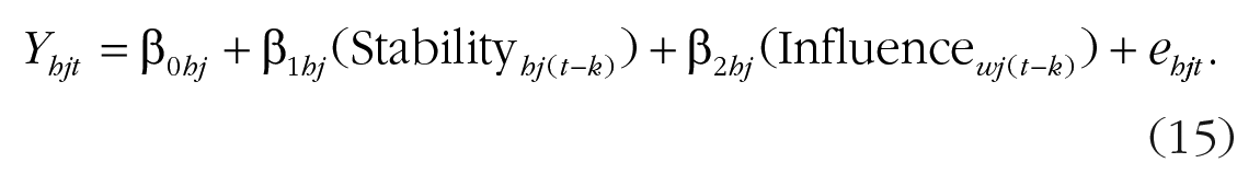
For distinguishable dyads, separate equations for each dyad member using a two-intercept approach are again estimated. With this model, one could test whether wives are more consistently tense over time than husbands (stability path) or whether wives are more or less influenced by their husbands’ tension than vice versa (influence path). Equations 14 and 15 represent the Level 1 equations:

$$Y_{wjt}={\mathrm{\beta }}_{0wj}+{\mathrm{\beta }}_{1wj}({\mathrm{Stability}}_{wj\left(t-k\right)})+{\mathrm{\beta }}_{2wj}({\mathrm{Influence}}_{hj\left(t-k\right)})+e_{wjt}$$ (14)

$$Y_{hjt}={\mathrm{\beta }}_{0hj}+{\mathrm{\beta }}_{1hj}({\mathrm{Stability}}_{hj(t-k)})+{\mathrm{\beta }}_{2hj}({\mathrm{Influence}}_{wj(t-k)})+e_{hjt}.$$ (15)

The Level 1 equation can be further broken down into Level 2 equations. ${\mathrm{\beta }}_{0wj}$ and ${\mathrm{\beta }}_{0hj}$ (Equations 16 and 17) represent the intercepts for wives and husbands in dyad $j$ , respectively. ${\mathrm{\beta }}_{1wj}$ (Equation 18) and ${\mathrm{\beta }}_{1hj}$ (Equation 19) represent their stability slopes, and ${\mathrm{\beta }}_{2wj}$ and ${\mathrm{\beta }}_{2hj}$ (Equation 16) are their influence slopes. The $\mathrm{\gamma }$ terms reflect the fixed intercepts and slopes across dyads, and the u terms capture dyad-level variability around those averages:

$${\mathrm{\beta }}_{0wj}={\mathrm{\gamma }}_{0w}+u_{0wj}$$ (16)

$${\mathrm{\beta }}_{0hj}={\mathrm{\gamma }}_{0h}+u_{0hj}$$ (17)

$${\mathrm{\beta }}_{1wj}={\mathrm{\gamma }}_{1w}+u_{1wj}$$ (18)

$${\mathrm{\beta }}_{1hj}={\mathrm{\gamma }}_{1h}+u_{1hj}$$ (19)

$${\mathrm{\beta }}_{2wj}={\mathrm{\gamma }}_{2w}+u_{2wj}$$ (20)

$${\mathrm{\beta }}_{2hj}={\mathrm{\gamma }}_{2h}+u_{2hj}.$$ (21)

Before specifying the model, researchers need to decide what the appropriate lag should be based on a combination of theoretical and empirical considerations. With any over-time data, it is important to consider how the variable of interest changes over time to determine the appropriate number of measurements and intervals between measurements to capture meaningful change (Dormann & Griffin, 2015; Hamaker, 2023). In the following exercise, we examine physiologic change measured in 30-s segments. Physiologic responses, such as heart rate variability (HRV), respond quickly, and change can be detected within 30 s (Helm et al., 2018). For this reason, it is common for researchers to examine change using 30-s segments with a lag of 1, assuming a consistent lag throughout (for a discussion of appropriate lags for physiologic data, see K. R. Thorson et al., 2018). As another practical note, the data frame should be in a person-period pairwise format such that each row represents one dyad member’s response at a specific time point in a long format alongside a column of the person’s own lagged response and the person’s partner’s lagged response. Thus, each row includes a variable that represents the current response (reactivity at time t), stability (reactivity at time t – k), and influence (the partner’s reactivity at time t – k), creating a “checkerboard” structure (see West, 2013).

Which statistics program should you use?

One important consideration is what program you plan to use to estimate the model. We start with SAS because it allows you to specify constraints on the variances and covariances, which is useful not only for pooling across dyad members for specific random effects (i.e., to treat dyad members as indistinguishable) but also for trimming out specific random effects. In the second half of the tutorial, we show how to adapt these analyses for R. Although R does not offer the same flexibility in specifying parameter constraints, it offers some advantages over SAS. For instance, it uses a different optimization method that can help complex models converge more easily. In that section, we discuss key differences between SAS and R that researchers should consider when selecting a software program. We now turn to best practices for specifying (and respecifying) random effects for dyadic longitudinal multilevel models.

Guidelines for Estimating Random Effects

With MLM, the goal is to achieve a balance between specifying a model that converges while retaining random effects that account for meaningful variance in the data. Our approach is guided by the best practices described in Figure 2. First, understand which random effects are necessary for the dyadic longitudinal model (Principle 1). For any type of over-time data for which there are time-varying variables that introduce nonindependence within persons, both random intercepts and random slopes should be included. Although the random intercept captures variability in the data, omitting the random slope forces all individuals to have the same pattern of change, which may not reflect the data (Principle 1a). In the same vein, ideally, all variances and covariances should be modeled. Excluding the covariances overlooks some of the interdependence in the data, such as how changes in dyad members’ responses are related, which is a core feature of dyadic data (Principle 1b). We discuss the implications of excluding the covariances in more detail later in the article. Once you have identified the random effects, the first analysis will be with the maximally specified random-effects model (Step 1), in which all possible variances and covariances are estimated. If the model fails to converge, that means the model was unable to reach a stable solution before reaching the maximum number of iterations (Peugh, 2010). This can occur when the model is overparameterized, such as when variances or covariances for some of the random effects are very small (near zero), the specified random effects structure is too complex relative to what the data can support (leading to overfitting or singularity), the sample size is small, or the optimization procedure is computationally limited (e.g., the algorithm reaches the iteration limit without finding a stable solution). To address these issues, the model parameters and/or optimization settings will need to be respecified.

Fig. 2.

Best practices for dyadic longitudinal multilevel models.

Before beginning the respecification process (i.e., moving onto Step 2), note that in SAS, you can set starting parameters, which often helps with convergence. These parameters act as initial guesses for the variances and covariances and are especially helpful when your random effects are small—something that happens often with complex models such as the stability and influence model. Very simply, convergence works from a starting point and then runs through iterations until the model reaches the best estimate. If the model’s starting point is too far from the actual parameter values, the model can struggle to converge. By setting starting values, you are essentially moving the starting line closer to the actual estimates, making it easier to find a solution. You can get these values from running a simpler version of the model, such as starting with the null model in which only the random effects are estimated or pulling values from similar models. Note that the number of starting values corresponds to the number of parameters. As an example, later in the article, we discuss the structure of the random effects for indistinguishable dyads (see Fig. 9). For this analysis, we are estimating 12 random effects (six variances and six covariances), one repeated effect to account for repeated observations in the dyad, and one residual variance, and therefore, we would need 14 starting parameters.

Even with starting values, the model still may not converge. If some random effects are near zero, including all random effects can overcomplicate the model, essentially asking it to estimate more than it reliably can. However, failing to include a random effect that exists—which implicitly sets the effect to zero—can lead to model misspecification, potentially biasing the fixed effects (Judd et al., 2012; see Principle 1). Understanding the source of nonconvergence involves both statistical and methodological considerations. Sometimes, the lack of variance in random effects can be traced back to the study design. For example, when tracking linguistic coordination between married couples during a conflict conversation, a researcher needs variability in how people adjust to their partner’s speaking style, adjusting for the stability in their own speaking style (Nasir et al., 2019). Linguistic coordination is calculated line by line, and if people’s speaking styles are too fixed—resembling a trait rather than a state that varies throughout the conversation—then all the variance will be between people, leaving little to model in the partner covariances (e.g., the degree to which one’s linguistic coordination is correlated with one’s partner’s linguistic coordination).

As another example, consider a study in which physiologic measures are collected to track changes in affect during an hour-long social interaction. The study design should allow for variability within and between individuals, capturing the fluxes and flows in people’s affective states (Brown et al., 2021; K. R. Thorson et al., 2018; West & Mendes, 2023). An optimal study would use a paradigm in which affect is expected to fluctuate, moving from stressed and tense, to happy and relaxed. This design allows researchers to model moment-to-moment shifts in affective intensity within the dyad. Because random effects are used to model variability, it is important that data have enough variability both between and within persons, which is a consideration that should be discussed at the design stage.

Begin the respecification process

If setting starting parameters does not help with model convergence, the next step is to begin the respecification process described in Step 2. There are three main options: (a) gradually trim the model, (b) build the model incrementally, or (c) use a simpler covariance structure. Following Step 2a, we recommend simplifying the random effects mostly likely to be near zero, starting with those that tend to be the smallest in prior work (e.g., between-persons-between-variables covariances; K. R. Thorson et al., 2018) and building up to those that are typically the largest (e.g., within-persons covariances). There are two ways to simplify the random-effects structure: pooling and trimming. Pooling means constraining certain parameters to be equal. For example, one might start by estimating separate random slopes for husbands and wives to capture differences in how each partner’s stress changes over time. Pooling these effects would set these parameters to be equal across partners, assuming that the rate of change in stress is the same for husbands and wives. Trimming, on the other hand, means removing a random effect from the model entirely. This sets the parameter to zero and assumes no variability in that effect. For example, trimming the random slope would imply that neither partner’s stress varies over time. Of these approaches, pooling is the more conservative option. Next, we walk through the respecification process and explain when each approach is most appropriate.

For distinguishable dyads, start by pooling the random effects you expect to be smallest and to contribute to nonconvergence before trimming them out completely (see Step 2a.i.). Pooling is often preferred over trimming because it retains the random effect, whereas trimming removes the parameter from the model entirely. For this reason, we recommend pooling as a first step. Pooling random effects does not eliminate all indicators of distinguishability. When working with distinguishable dyads, distinguishability can (and often should) be modeled in the fixed effects. If you start with a model that includes distinguishability in both the fixed and random effects and find yourself needing to simplify the random effects to achieve convergence, you should not also drop distinguishability from the fixed effects. In fact, the fixed effects should not be modified at all during the respecification process (see Principle 2). For example, in Model 4 of the stability and influence respecification exercise (Fig. 8), we constrain the partners’ random effects to be equal while preserving distinguishability in the fixed effects by modeling the effect of role (“partnum”). The goal of model respecification is to identify the random structure that best captures variability in the data while keeping the fixed effects constant. If changes are made to both the fixed and random effects, this can affect the model’s overall fit in ways that might be difficult to detect. When comparing models to determine the best fit, models using restricted estimation maximum likelihood can be compared only if they differ in their random effects; changes to the fixed effects require using maximum likelihood, which is considered more prone to bias (Ledermann & Kenny, 2017). Therefore, to determine the best model for your analyses, differences between models should involve only changes to the random effects (for a more in-depth discussion, see West, 2013). If the model still fails to converge after pooling, trimming covariances may be necessary.

If you are unsure of which covariances are contributing most to nonconvergence, we recommend following Step 2b: Start with the bare bones model, in which only the variances are included, and then build in the covariances incrementally. Following the same logic of Step 2a, start by pooling the covariances, and if that model converges, make them distinguishable. Continue this process until you encounter convergence issues. Then, repeat the specification process following Step 2a. As a reminder, do not use p values to decide what the final model should be. Instead, use theory and model convergence to guide your decisions. By building the model up and then systematically tearing it down, you can confidently identify which random effects should be included in the final model. If you are using a statistical program that does not allow you to create a user-specified variance-covariance matrix, you will need to skip to Step 2c: Simplify the random effects using a predefined covariance structure. We cover this approach in detail using R later in the tutorial.

Although this process is designed to help researchers find the optimal model, they may find themselves deciding between two models with different trade-offs. For example, imagine you have empirically distinguishable dyads—that is, you conducted a formal test of distinguishability (Kenny et al., 2006) and found that the variances between dyad members were indeed significantly different—and the model converges under two different specifications: (a) treating the dyads as indistinguishable at the level of the random effects but modeling all variances and covariances and (b) treating dyads as partially distinguishable, modeling separate variances for each partner but trimming some of the covariances. Although we generally recommend modeling as many random effects as the data allow—because trimming sets that effect is zero—the “best” model depends on both the research question and the data. First, how central is distinguishability to your design? If role differences are based on a subtle manipulation, such as one dyad member underwent an emotion induction and the other did not, you might accept a model that treats dyads as indistinguishable at the level of the random effects to preserve the full covariance matrix. If, however, the roles are fundamentally distinct, such as a terminally ill patient and the patient’s nurse, collapsing the random-effects structure would obfuscate meaningful and likely substantial between-roles differences. In this case, modeling dyads that are indistinguishable would be difficult to justify theoretically. Second, think about the dependent variable. Would you expect partners to differ drastically in variance on this outcome? For example, if you are modeling reaction time between an emotionally induced person and a neutral interaction partner, the variance by role might not be large enough to justify cutting out covariances for distinguishability in the variances. On the other hand, if you are modeling something such as life satisfaction in patient-nurse dyads, you would certainly expect substantial differences by role, and failing to account for distinguishability would not be in your best interest for both the theoretical question and empirical differences. Third, consider the other models you are running. Modeling some of the random effects as indistinguishable but not others would mean that the interpretation of the results would be inconsistent. Ultimately, our recommendation is to test both models and see which better represents the data. Are the covariances substantial or negligible? Does modeling distinguishable variances improve fit or clarify interpretation? These are the questions that should guide model selection, not the fixed effects. In fact, we caution against choosing models based on whether the fixed effects are significant because this opens the door to p-hacking. We revisit this model-selection dilemma in the respecification exercise in R, in which the options for variance-covariance matrices are much more limited.

In the following two sections, we demonstrate how to follow these guidelines for model specification using the dyadic growth-curve and stability and influence models for illustration. We present all syntax in SAS for distinguishable and indistinguishable dyads. Later in the article, we demonstrate how to adapt this code for R and compare output across programs. Given the challenges in adapting these analyses for indistinguishable dyads, we include only these results in the main article (all results for indistinguishable dyadic models are presented side-by-side in Tables 7 and 10). For the output for distinguishable dyads, see OSF (https://osf.io/yf9gq/?view_only=d079fb9d36aa444b88b2e8ed2144ec3a).

Model specification in SAS

Dyadic growth curve

We start with the dyadic growth-curve model based on Kenny and Ackerman (2023) using data from Campbell et al. (2005), in which 103 heterosexual couples reported their relationship satisfaction (“ASATISF”) over 14 days (“Time” was centered such that Time 0 represents Day 1). Partner gender is dummy-coded using the variables “man” and “woman” to distinguish between the dyad members. To model the main effect of partner gender and its interaction with time, we need to include only one of the dummy-coded variables (e.g., “man”) in the fixed effects. Given that the dyads are distinguishable, we start with a two-intercept model in which each dyad member is represented as the dyad members’ own random intercepts and random slopes, giving us four variables to include as random effects in the model (man, woman, Man × Time, Woman × Time). For this analysis, we are testing whether relationship satisfaction changes over time during a 2-week daily diary study and whether these changes differ between husbands and wives. Following Step 2, we estimate all variances and covariances (G matrix), resulting in 10 random effects total (see Fig. 3). This matrix is necessary for the user to set parameter constraints on the variance-covariance matrix. The matrix is “read” before the PROC MIXED syntax, which references the matrix. Note that specifying all variances and covariances is equivalent to using an unstructured variance-covariance matrix, which can be specified using “type = UN” in the random statement.

Fig. 3.

SAS syntax for specifying the G matrix using the dyadic growth-curve analysis with distinguishable dyads.

The unstructured model converged, and we do not need to further respecify the model. If the dyads are indistinguishable, the parameters in the model would initially be set equal across partners because dyad members are not theoretically distinct. This model starts with six random effects (Fig. 4).

Fig. 4.

SAS syntax for specifying the G matrix using the dyadic growth-curve analysis with indistinguishable dyads.

This exercise in SAS demonstrates the ideal case, in which the model converges for both distinguishable and indistinguishable models while estimating all variances and covariances. However, this will not always be the case. In the next section, we illustrate how to respecify the model when convergence fails using the stability and influence model. We then shift to R, starting with an overview of the key differences between SAS and R, followed by a simulation exercise that demonstrates how to address common convergence issues in the dyadic growth-curve model. Although we demonstrate dealing with nonconvergence using different models and statistical programs, how these respecification steps are implemented within each program applies across models.

Respecification exercise in SAS using the stability and influence model

To demonstrate the respecification process in action, we turn to the stability and influence model—a model notorious for its convergence issues. We are using a data set with 115 dyads (del Rosario et al., 2025). HRV was collected for 56 time points per person, scored in 30-s bins (28 min total). In total, there are 6,440 observations with 981 missing data points, leaving 5,459 observations in the analysis. In this model, we are testing whether one’s HRV from a prior time point (React_HRV_lagC) and one’s partner’s prior HRV (Partner_HRV_lagC) predict changes in HRV over time (React_HRV). The lagged variables represent HRV values from 30 s prior. Dyad members are represented by dummy variables I1 and I2, allowing us to test whether these effects differ by role. We start by treating the dyads as distinguishable, making it clear where in the process the guidelines apply to indistinguishable dyads.

Model 1: estimate all random effects

Following Step 1, we first try to estimate all random effects in the model using an unstructured variance-covariance matrix. The syntax for that model is provided in Figure 5 and has 21 random effects. This model did not converge. Given that we know which covariances tend to be the smallest for physiologic data (K. R. Thorson et al., 2018), we are following Step 2a for respecification: gradually simplify the model. Every step of the respecified model, including code, is presented in the respecification exercise below (Figs. 6–11).

Fig. 5.

Model 1: the stability and influence model for distinguishable dyads using G matrix in SAS.

Fig. 6.

SAS syntax for Model 2: pool the smallest covariances.

Fig. 7.

SAS syntax for Model 3: pool the larger covariances.

Fig. 8.

SAS syntax for Model 4: pool all variances and covariances.

Fig. 9.

SAS syntax for Model 5: trim out the smallest covariances.

Fig. 10.

SAS syntax for Model 6: build distinguishability back into the model.

Fig. 11.

SAS syntax for Model 7: trim out the remaining covariances.

Model 2: pool the smallest covariances

If the unstructured model—in which all variances and covariances are estimated and treated as distinguishable—does not converge, your first step is to pool the smallest covariances. For physiologic data, like in this data set, this tends to be the between-persons-between-variables covariances.

Model 3: pool the larger covariances

To further simplify Model 2, which pooled only the between-persons-between-variables covariances, Model 3 goes a step further by also pooling the within-persons covariances (Fig. 7, Lines 7–9). By pooling the within-persons covariances across dyad members, the model assumes that these relationships, such as the link between one person’s intercept and slope, are equivalent for both partners.

Model 4: pool all variances and covariances

If Model 3 does not converge, one can try pooling the variances, producing a model in which all the variances and covariances are constrained to be equal. The model now treats dyad members as indistinguishable at the level of the random effects.

Model 5: trim out the smallest covariances

If Model 4 does not converge, the next step is to simplify the random effects by removing parameters that are likely near zero and add unnecessary complexity to the model. In the context of the stability and influence model, this often means trimming the between-persons covariances, which are typically the smallest and least reliable. By removing these covariances, we reduce the number of parameters the model needs to estimate while preserving the within-persons covariances.

Model 6: build distinguishability back into the model

If Model 5 converges or Model 4 converged but your dyads are distinguishable, you can build distinguishability back into the model using Model 6. Here, the variances are distinguishable, and the remaining covariances are pooled. If Model 5 does not converge, move on to the next model.

Model 7: trim out the remaining covariances

If Model 5 does not converge, the final option is to trim the within-persons covariances (Fig. 11, Lines 4–6). This removes any remaining covariance terms and leaves only the variances for the intercept, stability slope, and influence slope.

In the respecification exercise (Figs. 5–11), we estimated seven different stability and influence models. We found that Model 4, in which all random effects were pooled, converged (Fig. 8). We continued the respecification exercise to demonstrate how distinguishability can be built back into the model after trimming. In Model 6 (Fig. 10), we made the variances distinguishable but not the covariances because doing so led to convergence failure. If you find that two models will converge—one that treats dyad members as distinguishable for some of the random effects (Model 6; Fig. 10) and another that treats them as indistinguishable for the same random effects (Model 5; Fig. 9)—we recommend you conduct a formal test of distinguishability to see if treating them as indistinguishable for those specific effects worsens the fit of the model. For guidelines on how to compare the relative fit of two models, see Peugh (2010) and West (2013). If the model fit worsens by pooling effects across the distinguishing factor (i.e., treating those effects as indistinguishable), then you should maintain distinguishability in those random effects.

Modifying these analyses for R

Up to this point, we have focused on SAS to illustrate model specification because it allows the creation of custom variance-covariance matrices. However, many researchers are turning to free software options, such as R. ¹ Although R offers many of the same statistical procedures as packages, there are some major limitations when it comes to longitudinal dyadic analysis. The main difference is that R does not allow the same level of flexibility with specifying the variance-covariance matrix. As we demonstrated, in SAS, you can start with the unstructured covariance matrix and then pool and/or trim whichever variances you want. In R, the options are more limited—you can specify a fully distinguishable model and estimate either all variances and covariances (unstructured covariance matrix) or just the variances (diagonal covariance matrix; see Step 2c). It is not currently possible to customize the covariance matrix using the nlme package (Version 3.1-164; Pinheiro et al., 2024) in RStudio (Version 4.2.2; RStudio Team, 2021), so to treat dyad members as indistinguishable, the sum-and-difference approach has to be used (see Kenny & Ackerman, 2023; Woody & Sadler, 2005).

Although these models are conceptually equivalent in SAS and R, differences in the software can lead to slightly different results. For example, the same analysis in SAS and R may use different approaches to calculate degrees of freedom. SAS uses the Satterthwaite method to estimate degrees of freedom, adjusting for unequal variances between groups and often resulting in fractional values. Although some MLM packages in R, such as lme4 (Bates et al., 2020), can implement the Satterthwaite method, nlme is generally more appropriate for dyadic analyses. This is because nlme accounts for two forms of nonindependence: random effects (G matrix) and correlated residuals (referred to as the “R matrix” in both R and SAS), which allows users to model nonindependence within dyad and over time. Moreover, nlme allows users to impose a covariance structure on the residuals to reflect the structure of the correlated residuals (e.g., unstructured, diagonal), which lme4 does not offer. However, the calculation of the degrees of freedom in nlme is limited to the following formula:

$$D{F}_i=m_i-(m_i-1+p_i),$$

where m_i is the number of groups at level $i$ and $p_i$ is the number of parameters at level $i$ . This approach partitions the variance across the levels of the model rather than adjusting for unequal variances, yielding a global estimate of the degrees of freedom for all fixed effects. Conversely, Satterthwaite estimation adjusts the degrees of freedom separately for each effect, depending on how they interact with the random effects, resulting in different degrees of freedom for each fixed effect.

Another major difference between programs is the optimization algorithm and convergence criteria. A model may converge with fewer (or more) iterations in R compared with SAS even when the exact same model is specified. Why? Because there are differences in how statistics programs handle random effects, especially when variance components are near zero, resulting in a model that is overfitted, which can lead to slight discrepancies in the results. In particular, nlme operates on an assumption of normality, and in turn, its algorithm is often more tolerant of small variance components and will estimate near-zero effects without flagging issues (Lu & Huang, 2014). SAS, on the other hand, will provide warnings when the model is close to overfitting. Warnings of near-zero variances are important because they suggest that the model may be overfitted, signaling that you may be trying to estimate a random effect that cannot be reliably estimated. We urge readers to be mindful of these differences between programs and ensure their data meet the model assumptions before beginning data analysis because failing to do so can lead to misleading results (Huang & Dagne, 2012). When small variances are not an issue, such as in the dyadic growth-curve data presented here, the programs yield the same results. For the stability and influence models, some random effects are near zero, which as we show, the programs handle very differently.

We begin by presenting R code for the dyadic growth-curve model using the same data set as before, starting with the approach for distinguishable dyads and then showing how this code can be adapted for indistinguishable dyads using the sum-and-difference method. Then, we simulate two data sets to demonstrate how respecification strategies differ between R and SAS in a dyadic growth-curve context. Finally, we return to the stability and influence model from the previous exercise and walk through how to fit it in R.

Dyadic growth-curve model in R

Distinguishable dyads

To build the starting model, we use an unstructured variance-covariance matrix by wrapping the random effects with pdSymm (this is the default; equivalent to UN in SAS). The code presented in Figure 12 is equivalent to Figure 3 from the previous exercise and produces the same results. Users can edit the convergence criteria by increasing the maximum number of iterations (maxIter in R and SAS) and the iterative method (niterEM in R; scoring in SAS), which helps the model stabilize and gives it more time to reach convergence. In this exercise, we use the same convergence criteria as we did in the previous SAS exercise. The model converged, and the output matches the model in SAS (for output comparison, see OSF: https://osf.io/yf9gq/?view_only=d079fb9d36aa444b88b2e8ed2144ec3a)

Fig. 12.

R Code for dyadic growth-curve model for distinguishable dyads.

Indistinguishable dyads

When working with indistinguishable dyads, it can be challenging to specify which variances and covariances should be pooled, especially when software limitations prevent specifying the covariance matrix beyond preset options, like in R. A useful workaround is the sum-and-difference approach (Kenny & Ackerman, 2023; Woody & Sadler, 2005). Instead of entering the random intercepts and slopes separately for each person, as we did for distinguishable dyads, the sum-and-difference method combines each dyad member’s intercepts and slopes to constrain partners to be equal. Just like the previous models, we designate one dyad member to be I1 and the other to be I2. Because dyad members are indistinguishable, there should be no meaningful difference between who is labeled “I1” and “I2.” We then use these dummy variables to compute a between-dyads and within-dyads effect, effectively “pooling” the partners’ random effects. For the between-dyads effect, we create a variable (ISum) representing the sum of the intercepts for I1 and I2 (Equation 22); the within-dyads effect (IDiff) is the difference between the intercepts (Equation 23; see Fig. 13 for the calculation in R):

$$I_{sijt}=M_{1ijt}+M_{2ijt}$$ (22)

$$I_{dijt}=M_{1ijt}-M_{2ijt}.$$ (23)

Fig. 13.

R code for dyadic growth-curve model for indistinguishable dyads using the sum-and-difference approach.

Next, we extend this approach to the slopes by multiplying the sum of the intercepts by time (TSum; Equation 24) and the difference between the intercepts by time (TDiff; Equation 25; Table 5):

$$T_{Su{m}_{ijt}}=\left(M_{1ijt}+M_{2ijt}\right)T_t$$ (24)

$$T_{Dif{f}_{ijt}}=\left(M_{1ijt}-M_{2ijt}\right)T_t.$$ (25)

Table 5.

Terms in Equations 22 through 25

Term	Description
$M_{1ijt}$	The intercept for Member 1 in dyad j at time t
$M_{2ijt}$	The intercept for Member 2 in dyad j at time t
Tt	The effect of time at time t
$I_{sijt}$	Sum of the intercepts for members of dyad j at time t
$I_{dijt}$	Difference between the intercepts for members of dyad j at time t
$T_{Sumij}$	Sum of time slopes (between-dyads effect) for dyad j at time t
$T_{Diffij}$	Difference in time slopes (within-dyads effect) for dyad j at time t

The sum-and-difference scores are then entered into the random statement of the mixed model as two separate blocks: one for the sum scores and one for the difference scores. By entering random effects into separate blocks using “pdBlocked” (Fig. 13), the random effects within each block correlate with one another while preventing correlations between the sum and the difference blocks. This setup is crucial because it reflects the conceptual distinction between the between-dyads effects (sum scores) and within-dyads effects (difference scores) and ensures that the variances for these effects are estimated independently. Note that this approach can also be used in SAS, in which case, separate RANDOM lines in PROC MIXED treats each set of sum and difference effects as “blocks.” The first block has the two sum variables (ISum and TSum), and the second block has the two difference variables (IDiff and TDiff). For brevity, we do not review the syntax for the sum-and-difference method in SAS, but the syntax is available on OSF (https://osf.io/yf9gq/?view_only=d079fb9d36aa444b88b2e8ed2144ec3a).

The output itself does not show the random-effects results. Instead, the variances and covariances will need to be manually calculated (for the code, see bottom of Fig. 13; for an overview of random-effects calculations, see Table 6). The code provided was adapted from Kenny and Ackerman (2023), which provides an in-depth discussion of the sum-and-difference method for dyadic growth-curve models.

Table 6.

Comparison of SAS G Matrix and R Sum-and-Difference Approach for Dyadic Growth Curve

Parameter	Computation details	Interpretation
Intercept variance	1 1 1 1 (P1 intercept)	How much do people vary in their perceived appreciation at baseline?
	1 2 2 1 (P2 intercept)
	ISum + IDiff
Slope variance	2 3 3 1 (P1 slope)	How much do people differ in their rate of change in appreciation over time?
	2 4 4 1 (P2 slope)
	TSum + TDiff
Within-persons intercept-slope covariance	3 1 3 1 (P1 intercept-stability)	Do people who begin feeling highly (or less) appreciated show increases (or declines) over time?
	3 2 4 1 (P2 intercept-stability)
	(ISum, TSum) + (IDiff, TDiff)
Between-persons intercept covariance	4 1 2 1 (P1 and P2 intercept covariance)	Do partners tend to start off feeling similarly appreciated?
	ISum – IDiff
Between-persons slope covariance	5 3 4 1 (P1 and P2 slope covariance)	Are partners’ rates of change in appreciation similar?
	TSum – TDiff
Between-persons intercept-slope covariance	6 1 4 1 (P1 intercept – P2 slope)	If one person starts with feeling appreciated, are there increases (or declines) in how appreciated the person’s partner feels over time?
	6 2 3 1 (P2 intercept – P1 slope)
	(ISum, TSum) – (IDiff, TDiff)

Note: Shaded areas represent the sum-and-difference equivalent. Expressions such as ISum + IDiff refer to the sum of variances (e.g., for intercepts or slopes). Expressions in parentheses, for example, (ISum, TSum), represent covariances between two random effects.

To illustrate the similarities and differences between approaches, we compared the output of three models: the G matrix in SAS and the sum-and-difference approach in R and SAS (for G matrix syntax, see Fig. 4; for results, see Tables 7 and 8). As we show, the results are consistent across programs and approaches.

Table 7.

Dyadic Growth-Curve Fixed Effects Comparing the G Matrix and Sum-and-Difference Methods

Method	Effect	b	SE	df	t	p
G matrix (SAS)	Intercept	6.2294	0.0686	102	90.86	< .0001
	Time	0.0145	0.0053	102	2.73	.0075
Sum and difference (SAS)	Intercept	6.2294	0.0686	102	90.86	< .0001
	Time	0.0145	0.0053	102	2.73	.0075
Sum and difference (R)	Intercept	6.2294	0.0686	2,762	90.86	< .0001
	Time	0.0145	0.0053	2,762	2.73	.0064

Note: Fixed effects are equivalent across methods. Degrees of freedom differ because of estimation procedure: SAS uses Satterthwaite approximation, and R uses model-based estimation.

Table 8.

Comparison of Model Respecification Output in R Using pdDiag and the Sum-and-Difference Approach

	Data Set 1		Data Set 2
Parameter	pdDiag	Sum and difference	pdDiag	Sum and difference
Fixed effects
Intercept	5.03 (0.07)	5.03 (0.08)	4.97 (0.02)	4.97 (0.05)
Time slope	−0.48 (0.03)	−0.48 (0.03)	0.55 (0.02)	0.55 (0.06)
Role (working)	2.09 (0.11)	2.09 (0.11)	−2.03 (0.08)	−2.03 (0.07)
Time × Role	0.33 (0.04)	0.33 (0.04)	0.30 (0.08)	0.30 (0.08)
Random effects
Intercept variance
Working parent	0.031	*0.061	0.028	*0.286
Stay-at-home parent	0.000		0.544
Slope variance
Working parent	0.000	*0.007	0.033	*0.334
Stay-at-home parent	0.000		0.634
Within-persons intercept-slope covariance	—	−0.018	—	−0.006
Between-persons intercept covariance	—	0.038	—	0.008
Between-persons slope covariance	—	0.007	—	−0.006
Between-persons intercept-slope   covariance	—	−0.019	—	0.001

*

Estimates are pooled across dyad members; Working and Stay-at-Home parents share the same value.

Model respecification exercise in R using the dyadic growth-curve model

Up to this point, we have demonstrated model specification for dealing with nonconvergence in SAS using the stability and influence model. Here, we apply the same logic in R using the dyadic growth-curve model. We use simulated data to systematically show how common issues in dyadic data, such as near-zero covariances, can lead to convergence problems and how researchers can troubleshoot while preserving the theoretically meaningful aspects of the model.

We begin by simulating dyadic longitudinal data (N = 100) with five waves of data. Each dyad represents new parents: one working parent and one stay-at-home parent. Given that these roles are theoretically distinguishable, we assume different fixed intercepts and slopes for each. The outcome variable is perceived appreciation, which we model as decreasing over time for both parents but to a greater degree for stay-at-home parents. In real dyadic data sets, issues such as low variability between dyad members or near-zero covariances are common. We walk through two examples to demonstrate how to handle these issues in R.

We simulate two data sets—one with near-zero between-persons covariances (i.e., intercept–intercept, slope–slope, P1 intercept–P2 slope, and P2 intercept–P1 slope) and the other with low variability between dyad members. For both data sets, the unstructured distinguishable model does not converge. The first step would be to revise the convergence criteria in the control argument by increasing the maximum number of iterations or changing the tolerance for convergence criteria via niterEM, msMaxIter, and tolerance (see lmecontrol function in the nlme package; Pinheiro et al., 2024). If the model still does not converge, we move to modifying the random-effects structure. In SAS, we would gradually simplify the model (Step 2a.i.), starting with pooling the between-persons covariances and then within-persons covariances, and if that does not work, we trim out covariances entirely. R, however, does not provide the same flexibility to pool and trim covariances incrementally. Instead, our two options are to (a) pool variances across the two dyad members (treating the dyads as indistinguishable; Model 4 in Fig. 8 of the respecification exercise in SAS) or (b) keep the variances distinguishable while trimming the covariances out entirely by switching from an unstructured (pdSymm) to a diagonal (pdDiag) covariance structure. The first option preserves the covariances but collapses the differences between partners’ variances, whereas the second option preserves variance differences but sacrifices the covariances. As discussed earlier, when given the option between pooling and trimming random effects, the former is generally preferred. However, this is not a one-size-fits-all solution, and the decision depends on the research question and data itself (for a more in-depth discussion on this topic, see section on model-specification guidelines for estimating random effects).

The choice between (a) pooling the variances and covariances or (b) trimming all covariances each have important trade-offs. Starting with the first option, if the dyads are statistically distinguishable—that is, you have tested for distinguishability and found significant differences in partner variances—then modeling the random effects as indistinguishable would ignore meaningful between-partners differences. However, this does not necessarily rule it out as an option. In the SAS respecification exercise, we followed Step 2a.i. of the model-specification guidelines and ended up with a model in which the variances and covariances were pooled across partners (Model 4 in Fig. 8). Even though dyad members were not empirically distinguishable in this data set, they were treated as such for the sake of illustration. We then provided the option of stopping there or building distinguishability back into the model, advising users to do both and compare the models. An important distinction is we arrived at that model through systematic pooling and trimming. Conversely, R limits users to an all-or-nothing approach—treating all random effects as either distinguishable or indistinguishable. In other words, simplifying to indistinguishable random effects can be justified, but if the ideal model for your data includes a mix of distinguishable and indistinguishable random effects, SAS would allow for this nuance, and R would not. Note that you can still test whether effects differ by role in the fixed effects even if the random effects are pooled.

If the unstructured model does not converge in R, the second option would be to keep separate variances for each partner by estimating a diagonal matrix (pdDiag), which models distinguishability in the variances but drops the covariances. Although the model still recognizes interdependence between partners by correlating their errors—within-dyads residual correlations are captured via corCompSymm—covariances are no longer included in the model. Without the covariances, the ability to estimate how partners’ trajectories covary in the random-effects structure is lost.

In this exercise, we use both respecification options across two data sets by trimming the covariances using pdDiag and treating the data as indistinguishable using the sum-and-difference approach (see Table 8). All random effects in Data Set 1 are very small, and there are some notable differences in variance between the roles in Data Set 2. As we show, pooling the variances between partners in this second analysis eliminates potentially meaningful differences between parents.

These examples illustrate how to follow the same model-specification process in R and how differences between programs inform those choices. Although we focus on modifying the model within a frequentist MLM perspective, there are alternative solutions that may be of interest to researchers, such as Bayesian estimation. Shifting from a frequentist to Bayesian approach, however, is not a one-to-one substitution. Bayesian estimation involves different assumptions and interpretations, and therefore, we do not present it as part of our model-specification guidelines. We do briefly touch on how researchers could move to that framework in our discussion of alternative approaches later in the article.

Stability and influence model in R

Distinguishable dyads

The setup for the stability and influence model in R is similar to the dyadic growth curve, but instead of time, we are modeling the effect of stability and influence as random slopes (Fig. 14). When we modeled these data as distinguishable in SAS, the model did not converge because of small variances. In fact, it did not converge until all parameters were pooled, treating the dyad members as indistinguishable (Fig. 8, Model 4). The unstructured model, however, did converge in nlme. A comparison of results is available in the supplemental material (https://osf.io/yf9gq/?view_only=d079fb9d36aa444b88b2e8ed2144ec3a).

Fig. 14.

R Code for stability and influence model for distinguishable dyads.

Indistinguishable dyads

For the stability and influence model with indistinguishable dyads, we will need to again use the sum-and-difference approach. We have six total random variables. In addition to ISum (Equation 26) and IDiff (Equation 27), we multiply the sum of the intercept $(M_{1ijt}+M_{2ijt})$ by lagged HRV $(A_{t-k})$ for stability ( $A_{Su{m}_{ijt}}$ ; HRVSum1; Equation 28) and by lagged partner HRV $(C_{t-k})$ for influence ( $C_{Su{m}_{ijt}}$ ; HRVSum2; Equation 29) for the between-dyads effects:

$$I_{sijt}=M_{1ijt}+M_{2ijt}$$ (26)

$$I_{dijt}=M_{1ijt}-M_{2ijt}$$ (27)

$$A_{Su{m}_{ijt}}=(M_{1ijt}+M_{2ijt})A_{t-k}$$ (28)

$$C_{Su{m}_{ijt}}=(M_{1ijt}+M_{2ijt})C_{t-k}.$$ (29)

We repeat this process for the within-dyads effects by multiplying the difference between the intercepts $(M_{1ijt}+M_{2ijt})$ by lagged HRV $(A_{t-k})$ for stability ( $A_{Dif{f}_{ijt}}$ ; HRVDiff1; Equation 30) and lagged partner HRV ( $C_{t-k}$ ) for influence ( $C_{Dif{f}_{ijt}}$ ; HRVDiff2; Equation 31; Table 9). See Table 10 for a conceptual comparison of random effects for indistinguishable dyads using the G matrix and sum-and-difference approach and Figure 15 for the sum-and-difference calculation in R:

$$A_{Dif{f}_{ijt}}=(M_{1ijt}-M_{2ijt})A_{t-k}$$ (30)

$$C_{Dif{f}_{ijt}}=(M_{1ijt}-M_{2ijt})C_{t-k}.$$ (31)

Table 9.

Terms in Equations 26 Through 31

Term	Description
$M_{1ijt}$	The intercept for Member 1 in dyad j at time t
$M_{2ijt}$	The intercept for Member 2 in dyad j at time t
$A_{t-k}$	The stability (autoregressive) effect of HRV at time t – k
$C_{t-k}$	The influence (cross-lagged) effect of HRV at time t – k
$I_{sijt}$	Sum of the intercepts for person i in dyad j at time t
$I_{dijt}$	Difference between the intercepts for person i in dyad j at time t
$A_{Su{m}_{ijt}}$	Stability slope sum (between-dyads effect) for person i in dyad j at time t
$C_{Su{m}_{ijt}}$	Influence slope sum (between-dyads effect) for person i in dyad j at time t
$A_{Dif{f}_{ijt}}$	Stability slope difference (within-dyads effect) for person i in dyad j at time t
$C_{Dif{f}_{ijt}}$	Influence slope difference (within-dyads effect) for person i in dyad j at time t

Note: HRV = heart-rate variability.

Table 10.

Comparison of SAS G Matrix and R Sum-and-Difference Approach for Indistinguishable Dyads

Parameter	Computation details	Interpretation
Intercept variance	1 1 1 1 (P1 intercept)	How much do people vary in their stress at baseline?
	1 2 2 1 (P2 intercept)
	ISum + IDiff
Stability slope variance	2 3 3 1 (P1 stability)	Do people vary in how stable their stress is?
	2 4 4 1 (P2 stability)
	HRVSum1 + HRVDiff1
Influence slope variance	3 5 5 1 (P1 influence	Do people vary in how much their stress is influenced by their partners?
	3 6 6 1 (P2 influence)
	HRVSum2 + HRVDiff2
Within-persons intercept-stability covariance	4 1 3 1 (P1 intercept-stability)	Are people with high baseline stress more or less stable in their stress?
	4 2 4 1 (P2 intercept-stability)
	(ISum, HRVSum1) + (IDiff, HRVDiff1)
Within-persons stability-influence covariance	6 3 5 1 (P1 stability-influence)	Is the stability of a person’s stress related to how influenced the person is by the person’s partner’s stress?
	6 4 6 1 (P2 stability-influence)
	(HRVSum1, HRVSum2) + (HRVDiff1, HRVDiff2)
Between-persons intercept covariance	7 1 2 1 (P1 and P2 intercept covariance)	Do partners tend to start off with similar stress levels?
	ISum - IDiff
Between-persons intercept-stability covariance	8 1 4 1 (P1 intercept – P2 stability)	Is one person’s baseline stress related to the stability of that person’s partner’s stress?
	8 2 3 1 (P2 intercept – P1 stability)
	(ISum, HRVSum1) – (IDiff, HRVDiff1)
Between-persons intercept-influence covariance	9 1 6 1 (P1 intercept – P2 influence)	Is one person’s baseline stress related to how strongly the person’s partner’s stress is influenced by the person?
	9 2 5 1 (P2 intercept – P1 influence)
	(ISum, HRVSum2) – (IDiff, HRVDiff2)
Between-persons stability-influence covariance	10 3 6 1 (P1 stability – P2 influence)	Is the stability of a person’s stress related to how much the person’s partner’s stress is influenced by the person?
	10 4 5 1 (P2 stability – P1 influence)
	(ISum, HRVSum1) – (IDiff, HRVDiff1)

Note: Shaded areas represent the sum-and-difference equivalent. Expressions such as ISum + IDiff refer to the sum of variances (e.g., for intercepts or slopes). Expressions in parentheses, such as (ISum, HRVSum1), represent covariances between two random effects.

Fig. 15.

R code for stability and influence model for indistinguishable dyads using the sum-and-difference approach.

To compare the indistinguishable model results between R and SAS, we ran three models: pooled variances and covariances using the G matrix in SAS, the sum-and-difference approach in SAS, and the sum-and-difference approach in R. For the first model, we initially used the SAS syntax presented in Figure 6 (Model 4), making the model fully indistinguishable by excluding the “partnum” variable from the fixed effects. This model did not converge in SAS until we added starting parameters (Fig. 16). In SAS, both the G matrix and sum-and-difference approaches with the starting parameters specified produced identical results (Figs. 16 and 17). However, nlme in R does not allow users to set starting parameters, and the results are slightly different compared with SAS (Table 11). As previously mentioned, nlme uses a different optimization method that is more tolerant of small random effects and unstable models compared with SAS, which tends to be more conservative. It is difficult to know exactly what is going on “under the hood” of these statistical programs. Therefore, we caution readers to be aware that when working with complex models, the output may differ slightly between programs.

Fig. 16.

SAS syntax for the indistinguishable model with starting parameters using the G-matrix approach.

Fig. 17.

SAS syntax for the indistinguishable model with using the sum-and-difference approach.

Table 11.

Fixed-Effects Output From the Stability and Influence Model Comparing the G Matrix and Sum-and-Difference Methods

Method	Effect	b	SE	df	t	p
G matrix (SAS)	Intercept	−0.0428	0.0525	99	−0.81	.4171
	React_HRV_lagC	0.0638	0.0155	111	4.11	< .0001
	Partner_HRV_lagC	−0.0059	0.0142	95.5	−0.41	.6802
Sum and difference (SAS)	Intercept	−0.0428	0.0525	99	−0.81	.4171
	React_HRV_lagC	0.0638	0.0155	111	4.11	< .0001
	Partner_HRV_lagC	−0.0059	0.0142	95.5	−0.41	.6803
Sum and difference (R)	Intercept	−0.0441	0.0523	5345	−0.84	.3999
	React_HRV_lagC	0.0607	0.0154	5345	3.95	.0001
	Partner_HRV_lagC	−0.0041	0.0147	5345	−0.28	.7820

Note: All models estimate fixed effects for baseline stress (intercept), autoregressive stability (React_HRV_lagC), and partner influence (Partner_HRV_lagC). Degrees of freedom differ because of estimation method.

Alternative approaches

Thus far, we have handled the issue of nonconvergence by adjusting the random effects and exploring how these analyses can be adapted for other programs. However, there are alternative analytic approaches that users can explore. One option is to adopt a Bayesian approach, which can sometimes handle small random effects more effectively. Bayesian estimation allows users to specify priors—beliefs about the likely range of parameters values—which can stabilize estimation by shrinking extreme values toward those priors (van de Schoot et al., 2017). This shrinkage can help models converge in cases in which traditional (i.e., frequentist) multilevel models fail because of near-zero covariances. For illustration, we performed a Bayesian estimation using the simulated Data Set 2 from the dyadic growth-curve model specification exercise in R. The corresponding code and output are available on OSF (https://osf.io/yf9gq/?view_only=d079fb9d36aa444b88b2e8ed2144ec3a).

Note that switching to a Bayesian framework changes both the interpretation of the results and the kinds of questions one can ask. Frequentist models test the probability of the observed data given the null hypothesis, whereas Bayesian inference evaluates the probability of a parameter given the data and prior beliefs (Moeyaert et al., 2017). In other words, frequentist models focus on whether the data provide enough evidence to reject the null hypothesis, whereas Bayesian approaches estimate the posterior distribution to quantify uncertainty about those values after observing the data (Flores et al., 2022). An important caveat is that convergence alone does not signify whether the model is valid. Poorly chosen or overly strong priors can distort the posterior, and weakly identified effects might look meaningful because of how dominant the prior is (Baldwin & Fellingham, 2013). As with any estimation framework, researchers should always inspect diagnostics when deciding on the best approach (Wagenmakers et al., 2018). Although this approach is beyond the scope of this article, for examples of using Bayesian models for longitudinal dyadic data, see Zee and Bolger (2020).

Users might also consider DSEM, which incorporates features of time-series modeling and latent variable analysis using an SEM framework (Asparouhov et al., 2018). DSEM can estimate complex longitudinal processes, such as autoregressive and cross-lagged paths, while also modeling latent traits and random effects. It can be particularly useful for estimating reciprocal influence between partners over time because it can account for both individual-level latent traits and within-persons dynamics. For example, DSEM can estimate time-varying actor and partner effects while allowing for autoregressive error structures and random slopes across dyads (Savord et al., 2023). These capabilities make it a powerful option for modeling interdependence over time. However, it is not without its limitations. DSEM often requires large sample sizes and complex syntax, and resources currently available on how to implement DSEM largely limit their analyses to Mplus. Until more open-source tools are available, DSEM for dyadic analysis may remain out of reach for many R users. For examples of DSEM applied to dyadic data, see Savord et al. (2023) and Goodboy et al. (2024).

Simulate data for model building

In the analyses presented, we used both real and simulated data to demonstrate the process of building models. We provide code in RMarkdown to simulate dyadic growth-curve data, in which users can control the variability both within and between participants and estimate separate fixed and random effects for each partner to adjust the degree of heterogeneity in each person’s growth trajectory. Users can also introduce different levels of missingness or simulate data sets with near-zero covariance (for code, see OSF).

Data simulation can be a useful exercise when designing a study, and the goal is to understand how different factors might influence the models you plan to use. For example, imagine a physiologic study for which you are deciding between using physiologic sensors that physically connected to the hardware via wires, which is dependable, or a Bluetooth option, which is convenient because it allows more movement, but it comes with a cost: more missing data. By simulating data with different amounts and patterns of missingness, you can assess how these factors affect your model and whether the costs (higher rates of missing data) outweigh the benefits (more convenient and allows more naturalistic movement). This approach can be particularly helpful for preregistering models and writing grant proposals because it allows you to demonstrate that your model is robust against various levels of missingness or response patterns. Moreover, data simulation can be used to test how other data characteristics—such as the degree of variability—affect the model and can alert you to other potential considerations before data collection begins.

Conclusion

In this tutorial, we introduced best practices for dyadic longitudinal multilevel models, including guiding principles and steps for model specification (Fig. 2). These guidelines are designed to help readers construct a model that captures variability in the data without overcomplicating the model. Starting with Principle 1, we emphasize the importance of identifying which random effects are empirically necessary and why including both random intercepts and slopes are needed for longitudinal data. We recommend that researchers start with the unstructured model (Step 1), estimating all variances and covariances. If convergence issues arise, Step 2 provides guidance on respecifying the model through three approaches: (a) simplifying the model by pooling and trimming the smallest random effects, (b) starting with a bare-bones model and gradually building the random effects in, and (c) for R users, using a simpler predefined covariance structure. We urge readers to focus solely on editing the random effects during the respecification process to maintain consistent fixed effects because simultaneous changes to fixed and random effects can obscure model fit (Principle 2). Finally, we encourage researchers to define and preregister their analysis plan in advance, for which, data simulation can be useful (Principle 3). By following these guidelines, researchers can systematically construct a robust and empirically sound model.

We demonstrated model specification with the dyadic growth-curve and the stability and influence models through two exercises, one in SAS, which is highly flexible with random-effect specification, and one in R, which requires a different approach but is a popular program for many researchers. We also provided an in-depth discussion of the sum-and-difference method as an alternative to applying parameter constraints to the G matrix in SAS and addressed potential caveats when deciding between statistical programs. In this tutorial, we provide a practical guide to building multilevel models for repeated-measures dyadic data, addressing common issues in data analysis, and demonstrating how these analyses can be adapted for different statistical programs. This tutorial serves as a starting point for researchers who want to better understand random effects for over-time dyadic analysis.