Tractable algorithms for strong admissibility

Abstract

Much like admissibility is the key concept underlying preferred semantics, strong admissibility is the key concept underlying grounded semantics, as membership of a strongly admissible set is sufficient to show membership of the grounded extension. As such, strongly admissible sets and labellings can be used as an explanation of membership of the grounded extension, as is for instance done in some of the proof procedures for grounded semantics. In the current paper, we present two polynomial algorithms for constructing relatively small strongly admissible labellings, with associated min–max numberings, for a particular argument. These labellings can be used as relatively small explanations for the argument’s membership of the grounded extension. Although our algorithms are not guaranteed to yield an absolute minimal strongly admissible labelling for the argument (as doing so would have implied an exponential complexity), our best performing algorithm yields results that are only marginally larger. Moreover, the runtime of this algorithm is an order of magnitude smaller than that of the existing approach for computing an absolute minimal strongly admissible labelling for a particular argument. As such, we believe that our algorithms can be of practical value in situations where the aim is to construct a minimal or near-minimal strongly admissible labelling in a time-efficient way.

1. Introduction

In formal argumentation, one would sometimes like to show that a particular argument is (credulously) accepted according to a particular argumentation semantics, without having to construct the entire extension the argument is contained in. For instance, to show that an argument is in a preferred extension, it is not necessary to construct the entire preferred extension. Instead, it is sufficient to construct a set of arguments that is admissible. Similarly, to show that an argument is in the grounded extension, it is not necessary to construct the entire grounded extension. Instead, it is sufficient to construct a set of arguments that is strongly admissible.

The concept of strong admissibility was introduced by Baroni and Giacomin [1] as one of the properties to describe and categorise argumentation semantics. It was subsequently studied by Caminada and Dunne [3,6] who further developed strong admissibility in both its set and labelling form. In particular, the strongly admissible sets (resp. labellings) were found to form a lattice with the empty set (resp. the all- $\mathtt{u}\mathtt{n}\mathtt{d}\mathtt{e}\mathtt{c}$ labelling) as its bottom element and the grounded extension (resp. the grounded labelling) as its top element [3,6].

As a strongly admissible set (labelling) can be used to explain that a particular argument is in the grounded extension (for instance, by using the discussion game of [4]) a relevant question is whether one can identify an expanation that is minimal. That is, given an argument A that is in the grounded extension, how can one obtain:

(1) a strongly admissible set that contains A, of which the number of arguments is minimal among all strongly admissible sets containing A, and

(2) a strongly admissible labelling that labels A $\mathtt{i}\mathtt{n}$ , of which the number of $\mathtt{i}\mathtt{n}$ and $\mathtt{o}\mathtt{u}\mathtt{t}$ labelled arguments (its size, cf. [7]) is minimal among all strongly admissible labellings that label A $\mathtt{i}\mathtt{n}$ .

It has been found that the problem of computing (1) is NP-hard [11, Theorem 2]1 whereas the verification problem of (2) is co-NP-complete [7, Theorem 2].2 Moreover, it has also been observed that even computing a c-approximation for the minimum size of a strongly admissible set for a given argument is NP-hard for every $c⩾1$ [11]. This is in sharp contrast with the complexity of the general verification problem of strong admissibility (i.e. verifying whether a set/labelling is strongly admissible, without the constraint that it also has to be minimal) which has been found to be polynomial [6].

The complexity results related to minimal strong admissibility pose a problem when the aim is to provide the user with a relatively small explanation of why a particular argument is in the grounded extension. For this, one can either apply an algorithmic approach that yields an absolute minimal explanation, but has a worst-case exponential runtime, or one can apply an algorithmic approach that has a less than exponential runtime, but does not come with any formal guarantees of how close the outcome is to an absolute minimal explanation [11]. The former approach is taken in [11]. The latter approach is taken in our current paper.

In the absence of a dedicated algorithm for strong admissibility, one may be tempted to simply apply an algorithm for computing the grounded extension or labelling instead (such as [12,13]) if the aim is to do the computation in polynomial time. Still, from the perspective of minimality, this would yield the absolute worst outcome, as the grounded extension (labelling) is the maximal strongly admissible set (labelling). In the current paper we therefore introduce an alternative algorithm which, like the grounded semantics algorithms, runs in polynomial time but tends to produce a strongly admissible set (resp. labelling) that is significantly smaller than the grounded extension (resp. labelling). As the complexity results from [11] prevent us from giving any theory-based guarantees regarding how close the outcome of the algorithm is to an absolute minimal strongly admissible set, we will instead assess the performance of the algorithm using a wide range of benchmark examples.

The remaining part of the current paper is structured as follows. First, in Section 2 we give a brief overview of the formal concepts used in the current paper, including that of a strongly admissible set and a strongly admissible labelling. In Section 3 we then proceed to provide the proposed algorithm, including the associated proofs of correctness. Then, in Section 4 we assess the performance of our approach, and compare it with the results yielded by the approach in [11] both in terms of outcome and runtime. We round off with a discussion of our findings in Section 5.

2. Preliminaries

In the current section, we briefly restate some of the basic concepts in formal argumentation theory, including strong admissibility. For current purposes, we restrict ourselves to finite argumentation frameworks.

Definition 1.

An argumentation framework is a pair $(Ar,att)$ where $Ar$ is a finite set of entities, called arguments, whose internal structure can be left unspecified, and $att$ is a binary relation on $Ar$ . For any $x,y\in Ar$ we say that x attacks y iff $(x,y)\in att$ .

As for notation, we use lower case letters at the end of the alphabet (such as x, y and z) to denote variables containing arguments, upper case letters at the end of the alphabet (such as X, Y and Z) to denote program variables containing arguments, and upper case letters at the start of the alphabet (such as A, B and C) to denote concrete instances of arguments.

When it comes to defining argumentation semantics, one can distinguish the extension approach and the labelling approach [5]. We start with the extensions approach.

Definition 2.

Let $(Ar,att)$ be an argumentation framework, $x\in Ar$ and $Args\subseteq Ar$ . We define $x^{+}$ as $\{y\in Ar|x\text{attacks}y\}$ , $x^{-}$ as $\{y\in Ar|y\text{attacks}x\}$ , ${Args}^{+}$ as $\bigcup \{x^{+}|x\in Args\}$ , and ${Args}^{-}$ as $\bigcup \{x^{-}|x\in Args\}$ . $Args$ is said to be conflict-free iff $Args\cap {Args}^{+}=\mathrm{\varnothing }$ . $Args$ is said to defend x iff $x^{-}\subseteq {Args}^{+}$ . The characteristic function $F:2^{Ar}\to 2^{Ar}$ is defined as $F(Args)=\{x|Args\text{defends}x\}$ .

Definition 3.

Let $(Ar,att)$ be an argumentation framework. $Args\subseteq Ar$ is

an admissible set iff $Args$ is conflict-free and $Args\subseteq F(Args)$

a complete extension iff $Args$ is conflict-free and $Args=F(Args)$

a grounded extension iff $Args$ is the smallest (w.r.t. ⊆) complete extension

a preferred extension iff $Args$ is a maximal (w.r.t. ⊆) complete extension

As mentioned in the introduction, the concept of strong admissibility was originally introduced by Baroni and Giacomin [1]. For current purposes we will apply the equivalent definition of Caminada [3,6].

Definition 4.

Let $(Ar,att)$ be an argumentation framework. $Args\subseteq Ar$ is strongly admissible iff every $x\in Args$ is defended by some ${Args}^{\prime }\subseteq Args\setminus \{x\}$ which in its turn is again strongly admissible.

Fig. 1.

An example of an argumentation framework.

As an example (taken from [6]), in the argumentation framework of Figure 1 the strongly admissible sets are $\mathrm{\varnothing }$ , $\{A\}$ , $\{A,C\}$ , $\{A,C,F\}$ , $\{D\}$ , $\{A,D\}$ , $\{A,C,D\}$ , $\{D,F\}$ , $\{A,D,F\}$ and $\{A,C,D,F\}$ , the latter also being the grounded extension. The set $\{A,C,F\}$ is strongly admissible as A is defended by $\mathrm{\varnothing }$ , C is defended by $\{A\}$ and F is defended by $\{A,C\}$ , each of which is a strongly admissible subset of $\{A,C,F\}$ not containing the argument it defends. Please notice that although the set $\{A,F\}$ defends argument C in $\{A,C,F\}$ , it is in its turn not strongly admissible (unlike $\{A\}$ ). Hence the requirement in Definition 4 for ${Args}^{\prime }$ to be a subset of $Args\setminus \{A\}$ . We also observe that although $\{C,H\}$ is an admissible set, it is not a strongly admissible set, since no subset of $\{C,H\}\setminus \{H\}$ defends H.

It can be shown that each strongly admissible set is conflict-free and admissible [6]. The strongly admissible sets form a lattice (w.r.t. ⊆), of which the empty set is the bottom element and the grounded extension is the top element [6].

The above definitions essentially follow the extension based approach as described in [10]. It is also possible to define the key argumentation concepts in terms of argument labellings [2,8].

Definition 5.

Let $(Ar,att)$ be an argumentation framework. An argument labelling is a function $\mathcal{L}ab:Ar\to \{\mathtt{i}\mathtt{n},\mathtt{o}\mathtt{u}\mathtt{t},\mathtt{u}\mathtt{n}\mathtt{d}\mathtt{e}\mathtt{c}\}$ . An argument labelling is called an admissible labelling iff for each $x\in Ar$ it holds that:

if $\mathcal{L}ab(x)=\mathtt{i}\mathtt{n}$ then for each y that attacks x it holds that $\mathcal{L}ab(y)=\mathtt{o}\mathtt{u}\mathtt{t}$

if $\mathcal{L}ab(x)=\mathtt{o}\mathtt{u}\mathtt{t}$ then there exists a y that attacks x such that $\mathcal{L}ab(y)=\mathtt{i}\mathtt{n}$

$\mathcal{L}ab$ is called a complete labelling iff it is an admissible labelling and for each $x\in Ar$ it also holds that:

• if $\mathcal{L}ab(x)=\mathtt{u}\mathtt{n}\mathtt{d}\mathtt{e}\mathtt{c}$ then there is a y that attacks x such that $\mathcal{L}ab(y)=\mathtt{u}\mathtt{n}\mathtt{d}\mathtt{e}\mathtt{c}$ , and for each y that attacks x such that $\mathcal{L}ab(y)\ne \mathtt{u}\mathtt{n}\mathtt{d}\mathtt{e}\mathtt{c}$ it holds that $\mathcal{L}ab(y)=\mathtt{o}\mathtt{u}\mathtt{t}$

As a labelling is essentially a function, we sometimes write it as a set of pairs. Also, if $\mathcal{L}ab$ is a labelling, we write $\mathtt{i}\mathtt{n}(\mathcal{L}ab)$ for $\{x\in Ar|\mathcal{L}ab(x)=\mathtt{i}\mathtt{n}\}$ , $\mathtt{o}\mathtt{u}\mathtt{t}(\mathcal{L}ab)$ for $\{x\in Ar|\mathcal{L}ab(x)=\mathtt{o}\mathtt{u}\mathtt{t}\}$ and $\mathtt{u}\mathtt{n}\mathtt{d}\mathtt{e}\mathtt{c}(\mathcal{L}ab)$ for $\{x\in Ar|\mathcal{L}ab(x)=\mathtt{u}\mathtt{n}\mathtt{d}\mathtt{e}\mathtt{c}\}$ . As a labelling is also a partition of the arguments into sets of $\mathtt{i}\mathtt{n}$ -labelled arguments, $\mathtt{o}\mathtt{u}\mathtt{t}$ -labelled arguments and $\mathtt{u}\mathtt{n}\mathtt{d}\mathtt{e}\mathtt{c}$ -labelled arguments, we sometimes write it as a triplet $(\mathtt{i}\mathtt{n}(\mathcal{L}ab),\mathtt{o}\mathtt{u}\mathtt{t}(\mathcal{L}ab),\mathtt{u}\mathtt{n}\mathtt{d}\mathtt{e}\mathtt{c}(\mathcal{L}ab))$ .

Definition 6 ([9])

Let $\mathcal{L}ab$ and $\mathcal{L}{ab}^{\prime }$ be argument labellings of argumentation framework $(Ar,att)$ . We say that $\mathcal{L}ab⊑\mathcal{L}a{b}^{\prime }$ iff $\mathtt{i}\mathtt{n}(\mathcal{L}ab)\subseteq \mathtt{i}\mathtt{n}(\mathcal{L}a{b}^{\prime })$ and $\mathtt{o}\mathtt{u}\mathtt{t}(\mathcal{L}ab)\subseteq \mathtt{o}\mathtt{u}\mathtt{t}(\mathcal{L}a{b}^{\prime })$ .

Definition 7.

Let $\mathcal{L}ab$ be a complete labelling of argumentation framework $(Ar,att)$ . $\mathcal{L}ab$ is said to be

the grounded labelling iff $\mathcal{L}ab$ is the (unique) smallest (w.r.t. ⊑) complete labelling

a preferred labelling iff $\mathcal{L}ab$ is a maximal (w.r.t. ⊑) complete labelling

We refer to the size of a labelling $\mathcal{L}ab$ as $|\mathtt{i}\mathtt{n}(\mathcal{L}ab)\cup \mathtt{o}\mathtt{u}\mathtt{t}(\mathcal{L}ab)|$ . We observe that if $\mathcal{L}ab⊑\mathcal{L}a{b}^{\prime }$ then the size of $\mathcal{L}ab$ is smaller or equal to the size of $\mathcal{L}{ab}^{\prime }$ , but not necessarily vice versa. In the remainder of the current paper, we use the terms smaller, bigger, minimal and maximal in relation to the size of the respective labellings, unless stated otherwise.

The next step is to define a strongly admissible labelling. In order to do so, we need the concept of a min-max numbering [6].

Definition 8.

Let $\mathcal{L}ab$ be an admissible labelling of argumentation framework $(Ar,att)$ . A min-max numbering is a total function ${\mathcal{M}\mathcal{M}}_{\mathcal{L}ab}:\mathtt{i}\mathtt{n}(\mathcal{L}ab)\cup \mathtt{o}\mathtt{u}\mathtt{t}(\mathcal{L}ab)\to \mathbb{N}\cup \{\mathrm{\infty }\}$ such that for each $x\in \mathtt{i}\mathtt{n}(\mathcal{L}ab)\cup \mathtt{o}\mathtt{u}\mathtt{t}(\mathcal{L}ab)$ it holds that:

if $\mathcal{L}ab(x)=\mathtt{i}\mathtt{n}$ then ${\mathcal{M}\mathcal{M}}_{\mathcal{L}ab}(x)=max(\{{\mathcal{M}\mathcal{M}}_{\mathcal{L}ab}(y)|y\text{attacks}x\text{and}\mathcal{L}ab(y)=\mathtt{o}\mathtt{u}\mathtt{t}\})+1$ (with $max(\mathrm{\varnothing })$ defined as 0)

if $\mathcal{L}ab(x)=\mathtt{o}\mathtt{u}\mathtt{t}$ then ${\mathcal{M}\mathcal{M}}_{\mathcal{L}ab}(x)=min(\{{\mathcal{M}\mathcal{M}}_{\mathcal{L}ab}(y)|y\text{attacks}x\text{and}\mathcal{L}ab(y)=\mathtt{i}\mathtt{n}\})+1$ (with $min(\mathrm{\varnothing })$ defined as ∞)

It has been proved that every admissible labelling has a unique min-max numbering [6]. A strongly admissible labelling can then be defined as follows [6].

Definition 9.

A strongly admissible labelling is an admissible labelling whose min-max numbering yields natural numbers only (so no argument is numbered ∞).

As an example (taken from [6]), consider again the argumentation framework of Figure 1. Here, the admissible labelling $\mathcal{L}{ab}_1=(\{A,C,F,G\},\{B,E,H\},\{D\})$ has min-max numbering $\{(A:1),(B:2),(C:3),(E:4),(F:5),(G:\mathrm{\infty }),(H:\mathrm{\infty })\}$ , which means that it is not strongly admissible. The admissible labelling $\mathcal{L}{ab}_2=(\{A,C,D,F\},\{B,E\},\{G,H\})$ has min-max numbering $\{(A:1),(B:2),(C:3),(D:1),(E:2),(F:3)\}$ , which means that it is strongly admissible.

It has been shown that the strongly admissible labellings form a lattice (w.r.t. ⊑), of which the all- $\mathtt{u}\mathtt{n}\mathtt{d}\mathtt{e}\mathtt{c}$ labelling is the bottom element and the grounded labelling is the top element [6].

The relationship between extensions and labellings has been well-studied [2,8]. A common way to relate extensions to labellings is through the functions $\mathtt{A}\mathtt{r}\mathtt{g}\mathtt{s}\mathtt{2}\mathtt{L}\mathtt{a}\mathtt{b}$ and $\mathtt{L}\mathtt{a}\mathtt{b}\mathtt{2}\mathtt{A}\mathtt{r}\mathtt{g}\mathtt{s}$ . These translate a conflict-free set of arguments to an argument labelling, and an argument labelling to a set of arguments, respectively. More specifically, given an argumentation framework $(Ar,att)$ , and an associated conflict-free set of arguments $Args$ and a labelling $\mathcal{L}ab$ , $\mathtt{A}\mathtt{r}\mathtt{g}\mathtt{s}\mathtt{2}\mathtt{L}\mathtt{a}\mathtt{b}(Args)$ is defined as $(Args,{Args}^{+},Ar\setminus (Args\cup {Args}^{+}))$ and $\mathtt{L}\mathtt{a}\mathtt{b}\mathtt{2}\mathtt{A}\mathtt{r}\mathtt{g}\mathtt{s}(\mathcal{L}ab)$ is defined as $\mathtt{i}\mathtt{n}(\mathcal{L}ab)$ . It has been proven [8] that if $Args$ is an admissible set (resp. a complete, grounded or preferred extension) then $\mathtt{A}\mathtt{r}\mathtt{g}\mathtt{s}\mathtt{2}\mathtt{L}\mathtt{a}\mathtt{b}(Args)$ is an admissible labelling (resp. a complete, grounded or preferred labelling), and that if $\mathcal{L}ab$ is an admissible labelling (resp. a complete, grounded or preferred labelling) then $\mathtt{L}\mathtt{a}\mathtt{b}\mathtt{2}\mathtt{A}\mathtt{r}\mathtt{g}\mathtt{s}(\mathcal{L}ab)$ is an admissible set (resp. a complete, grounded or preferred extension). It has also been proven [6] that if $Args$ is a strongly admissible set then $\mathtt{A}\mathtt{r}\mathtt{g}\mathtt{s}\mathtt{2}\mathtt{L}\mathtt{a}\mathtt{b}(Args)$ is a strongly admissible labelling, and that if $\mathcal{L}ab$ is a strongly admissible labelling then $\mathtt{L}\mathtt{a}\mathtt{b}\mathtt{2}\mathtt{A}\mathtt{r}\mathtt{g}\mathtt{s}(\mathcal{L}ab)$ is a strongly admissible set.

3. The algorithms

In the current section, we present an algorithmic approach for computing a relatively small3 strongly admissible labelling. For this, we provide three different algorithms. The first algorithm (Algorithm 1) basically constructs a strongly admissible labelling bottom-up, starting with the arguments that have no attackers and continuing until the main argument (the argument for which one want to show membership of a strongly admissible set) is labelled $\mathtt{i}\mathtt{n}$ . The second algorithm (Algorithm 2) then takes the output of the first algorithm and tries to prune it. That is, it tries to identify only those $\mathtt{i}\mathtt{n}$ and $\mathtt{o}\mathtt{u}\mathtt{t}$ labelled arguments that are actually needed in the strongly admissible labelling. The third algorithm (Algorithm 3) then combines Algorithm 1 (which is used as the construction phase) and Algorithm 2 (which is used as the pruning phase). Overall, we assume that it has already been established that the main argument is in the grounded extension and that the aim is merely to find a (relatively small) explanation for this.

3.1. Algorithm 1

The basic idea of Algorithm 1 is to start constructing the grounded labelling bottom-up, until we reach the main argument (that is, until we reach the argument that we are trying to construct a strongly admissible labelling for; this argument should hence be labelled $\mathtt{i}\mathtt{n}$ ). As such, the idea is to take an algorithm for computing the grounded labelling (e.g. [12] or [13]) and modify it accordingly. We have chosen the algorithm of [13] for this purpose, as it has been proved to run faster than some of the alternatives (such as [12]). We had to adjust this algorithm in two ways. First, as mentioned above, we want the algorithm to stop once it hits the main argument, instead of continuing to construct the entire grounded labelling. Second, we want it to compute not just the strongly admissible labelling itself, but also its associated min-max numbering.

Obtaining the min-max numbering is important, as it can be used to show that the obtained admissible labelling is indeed strongly admissible, through the absence of ∞ in its min-max numbering. Additionally, the min-max numbering is also needed for some of the applications of strong admissibility, in particular the Grounded Discussion Game [4] where the combination of a strongly admissible labelling and its associated min-max numbering serves as a roadmap for obtaining a winning strategy.

Instead of first computing the strongly admissible labelling and then proceeding to compute the min-max numbering, we want to compute both the strongly admissible labelling and the min-max numbering in just a single pass, in order to achieve the best performance.

To see how the algorithm works, consider again the argumentation framework of Figure 1. Let C be the main argument. At the start of the first iteration of the while loop (line 21) it holds that $\mathcal{L}ab=(\{A,D\},\mathrm{\varnothing },\{B,C,E,F,G,H\})$ , ${\mathcal{M}\mathcal{M}}_{\mathcal{L}ab}=\{(A:1),(D:1)\}$ and $\mathtt{u}\mathtt{n}\mathtt{p}\mathtt{r}\mathtt{o}\mathtt{c}\mathrm{\_}\mathtt{i}\mathtt{n}=[A,D]$ . At the first iteration of the while loop, the argument in front of $\mathtt{u}\mathtt{n}\mathtt{p}\mathtt{r}\mathtt{o}\mathtt{c}\mathrm{\_}\mathtt{i}\mathtt{n}$ (A) is selected (line 22). This then means that B gets labelled $\mathtt{o}\mathtt{u}\mathtt{t}$ and C gets labelled $\mathtt{i}\mathtt{n}$ . Hence, the algorithm hits the main argument (C) at line 33 and terminates. This yields a labelling $\mathcal{L}ab=(\{A,C,D\},\{B\},\{E,F,G,H\})$ and associated min-max numbering ${\mathcal{M}\mathcal{M}}_{\mathcal{L}ab}=\{(A:1),(B:2),(C:3),(D:1)\}$ .

We now proceed to prove some of the formal properties of the algorithm. The first property to be proved is termination.

Theorem 1.

Let $AF=(Ar,att)$ be an argumentation framework and A be an argument in the grounded extension of $AF$ . Let both $AF$ and A be given as input to Algorithm 1. It holds that the algorithm terminates.

Proof.

As for the first loop (the for loop of lines 9–18) we observe that it terminates as the number of arguments in Ar is finite.

As for the second loop (the while loop of lines 21–37) we first observe that no argument can be added to unproc_in more than once (that is, once an argument has been added to unproc_in, it can never be added again). This is because for an argument to be added, it has to be labelled $\mathtt{u}\mathtt{n}\mathtt{d}\mathtt{e}\mathtt{c}$ (line 27) whereas after adding it, it will be labelled $\mathtt{i}\mathtt{n}$ (line 31). Moreover, once an argument is labelled $\mathtt{i}\mathtt{n}$ , it will never be labelled $\mathtt{u}\mathtt{n}\mathtt{d}\mathtt{e}\mathtt{c}$ again and therefore cannot be added to $\mathtt{u}\mathtt{n}\mathtt{p}\mathtt{r}\mathtt{o}\mathtt{c}\mathrm{\_}\mathtt{i}\mathtt{n}$ again. Given that (1) there is only a finite number of arguments in $Ar$ , (2) each argument can be added to unproc_in at most once, and (3) each iteration of the while loop removes an argument from unproc_in, it follows that the loop has to terminate.

Next, we need to show that the algorithm is correct. That is, we need to show that the algorithm yields a strongly admissible labelling $\mathcal{L}ab$ that labels A $\mathtt{i}\mathtt{n}$ , together with its associated min-max numbering ${\mathcal{M}\mathcal{M}}_{\mathcal{L}ab}$ . In order to do so, we first need to state and prove a number of lemmas. We start with showing that $\mathcal{L}ab$ is admissible in every stage of the algorithm.

Lemma 2.

Let $AF=(Ar,att)$ be an argumentation framework and A be an argument in the grounded extension of $AF$ . Let both $AF$ and A be given as input to Algorithm 1. It holds that during any stage in the algorithm, $\mathcal{L}ab$ is an admissible labelling.

Proof.

Consider the value of $\mathcal{L}ab$ at an arbitrary point during the execution of Algorithm 1. According to the definition of an admissible labelling (Definition 5) we need to prove two things, for an arbitrary argument $x\in Ar$ :

• (1)

if $\mathcal{L}ab(x)=\mathtt{i}\mathtt{n}$ then for each y that attacks x it holds that $\mathcal{L}ab(y)=\mathtt{o}\mathtt{u}\mathtt{t}$

Suppose $\mathcal{L}ab(x)=\mathtt{i}\mathtt{n}$ . We distinguish two cases:

• (a)

  x was labelled $\mathtt{i}\mathtt{n}$ at line 14. This implies that $\mathtt{u}\mathtt{n}\mathtt{d}\mathrm{\_}\mathtt{p}\mathtt{r}\mathtt{e}(x)=0$ in line 12, which implies that x has no attackers. Therefore, trivially $\mathcal{L}ab(y)=\mathtt{o}\mathtt{u}\mathtt{t}$ for each $y\in Ar$ that attacks x.

• (b)

  x was labelled $\mathtt{i}\mathtt{n}$ at line 31. This implies that $\mathtt{u}\mathtt{n}\mathtt{d}\mathtt{e}\mathtt{c}\mathrm{\_}\mathtt{p}\mathtt{r}\mathtt{e}(x)=0$ in line 29, which implies that each attacker y of x has been relabelled to $\mathtt{o}\mathtt{u}\mathtt{t}$ . To see that this is the case, let n be the number of attackers of x (that is, $n=|x^{-}|$ ). It follows that $\mathtt{u}\mathtt{n}\mathtt{d}\mathtt{e}\mathtt{c}\mathrm{\_}\mathtt{p}\mathtt{r}\mathtt{e}(x)$ is initially n (line 11) and at least 1 (otherwise x would have been labelled $\mathtt{i}\mathtt{n}$ at line 14 instead of at line 31). In order for $\mathtt{u}\mathtt{n}\mathtt{d}\mathtt{e}\mathtt{c}\mathrm{\_}\mathtt{p}\mathtt{r}\mathtt{e}(x)$ to have fallen to 0 (line 29) it will need to have decremented (at line 28) n times (as no other line changes the value of $\mathtt{u}\mathtt{n}\mathtt{d}\mathtt{e}\mathtt{c}\mathrm{\_}\mathtt{p}\mathtt{r}\mathtt{e}(x)$ ). Each time this happens at line 28, an attacker of x that wasn’t previously labelled $\mathtt{o}\mathtt{u}\mathtt{t}$ (line 24) is labelled $\mathtt{o}\mathtt{u}\mathtt{t}$ (line 25). Therefore, by the time $\mathtt{u}\mathtt{n}\mathtt{d}\mathtt{e}\mathtt{c}\mathrm{\_}\mathtt{p}\mathtt{r}\mathtt{e}(x)$ became 0, it follows that all attackers of x have become labelled $\mathtt{o}\mathtt{u}\mathtt{t}$ .

(2)

if $\mathcal{L}ab(x)=\mathtt{o}\mathtt{u}\mathtt{t}$ then there exists a y that attacks x such that $\mathcal{L}ab(y)=\mathtt{i}\mathtt{n}$

Suppose $\mathcal{L}ab(x)=\mathtt{o}\mathtt{u}\mathtt{t}$ . This implies that x was labelled $\mathtt{o}\mathtt{u}\mathtt{t}$ at line 25, which implies that an attacker y of x was an element of $\mathtt{u}\mathtt{n}\mathtt{p}\mathtt{r}\mathtt{o}\mathtt{c}\mathrm{\_}\mathtt{i}\mathtt{n}$ . This means that at some point, argument y was added to $\mathtt{u}\mathtt{n}\mathtt{p}\mathtt{r}\mathtt{o}\mathtt{c}\mathrm{\_}\mathtt{i}\mathtt{n}$ . This could have happened at line 13 or 30. In both cases, it follows that (line 14 and 31) y is labelled $\mathtt{i}\mathtt{n}$ .

The next lemma presents an intermediary result that will be needed further on in the proofs.

Lemma 3.

Let $AF=(Ar,att)$ be an argumentation framework and A be an argument in the grounded extension of $AF$ . Let both $AF$ and A be given as input to Algorithm 1. It holds that for each argument x that is added to $\mathtt{u}\mathtt{n}\mathtt{p}\mathtt{r}\mathtt{o}\mathtt{c}\mathrm{\_}\mathtt{i}\mathtt{n}$ , ${\mathcal{M}\mathcal{M}}_{\mathcal{L}ab}(x)⩾1$

Proof.

We prove this by induction over the number of arguments that are added to $\mathtt{u}\mathtt{n}\mathtt{p}\mathtt{r}\mathtt{o}\mathtt{c}\mathrm{\_}\mathtt{i}\mathtt{n}$ during the execution of the while loop of lines 21–37. BASIS (n = 0)

Suppose the while loop has not yet added any arguments to $\mathtt{u}\mathtt{n}\mathtt{p}\mathtt{r}\mathtt{o}\mathtt{c}\mathrm{\_}\mathtt{i}\mathtt{n}$ . This means that any argument x that was added to $\mathtt{u}\mathtt{n}\mathtt{p}\mathtt{r}\mathtt{o}\mathtt{c}\mathrm{\_}\mathtt{i}\mathtt{n}$ was added by the for loop (lines 9–18). This could only have been done at line 13. Line 15 then implies that ${\mathcal{M}\mathcal{M}}_{\mathcal{L}ab}(x)=1$ so trivially ${\mathcal{M}\mathcal{M}}_{\mathcal{L}ab}(x)⩾1$ .

STEP

Suppose that at a particular point, the while loop has added n ( $⩾0$ ) arguments to $\mathtt{u}\mathtt{n}\mathtt{p}\mathtt{r}\mathtt{o}\mathtt{c}\mathrm{\_}\mathtt{i}\mathtt{n}$ and that for each argument x that has been added to $\mathtt{u}\mathtt{n}\mathtt{p}\mathtt{r}\mathtt{o}\mathtt{c}\mathrm{\_}\mathtt{i}\mathtt{n}$ (either by the while loop of lines 21–37 or by the for loop of lines 9–18) it holds that ${\mathcal{M}\mathcal{M}}_{\mathcal{L}ab}(x)⩾1$ . We distinguish two cases:

x was added to $\mathtt{u}\mathtt{n}\mathtt{p}\mathtt{r}\mathtt{o}\mathtt{c}\mathrm{\_}\mathtt{i}\mathtt{n}$ previously. From the induction hypothesis it follows that ${\mathcal{M}\mathcal{M}}_{\mathcal{L}ab}(x)⩾1$ at the moment x was added. As Algorithm 1 does not change any value of ${\mathcal{M}\mathcal{M}}_{\mathcal{L}ab}$ once it is assigned, it follows that ${\mathcal{M}\mathcal{M}}_{\mathcal{L}ab}(x)⩾1$ still holds at the current point.

x is the argument that is currently being added to $\mathtt{u}\mathtt{n}\mathtt{p}\mathtt{r}\mathtt{o}\mathtt{c}\mathrm{\_}\mathtt{i}\mathtt{n}$ (so $x=Z$ at line 30). This implies that Z is labelled $\mathtt{i}\mathtt{n}$ at line 31 and is numbered ${\mathcal{M}\mathcal{M}}_{\mathcal{L}ab}(Y)+1$ at line 32. Following line 26, it holds that ${\mathcal{M}\mathcal{M}}_{\mathcal{L}ab}(Y)={\mathcal{M}\mathcal{M}}_{\mathcal{L}ab}(X)+1$ , with X being an $\mathtt{i}\mathtt{n}$ labelled attacker of Y that was added to $\mathtt{u}\mathtt{n}\mathtt{p}\mathtt{r}\mathtt{o}\mathtt{c}\mathrm{\_}\mathtt{i}\mathtt{n}$ previously. We can therefore apply the induction hypothesis and obtain that ${\mathcal{M}\mathcal{M}}_{\mathcal{L}ab}(X)⩾1$ , which together with the earlier observed facts that ${\mathcal{M}\mathcal{M}}_{\mathcal{L}ab}(Z)={\mathcal{M}\mathcal{M}}_{\mathcal{L}ab}(Y)+1$ (line 32) and ${\mathcal{M}\mathcal{M}}_{\mathcal{L}ab}(Y)={\mathcal{M}\mathcal{M}}_{\mathcal{L}ab}(X)+1$ (line 26) implies that ${\mathcal{M}\mathcal{M}}_{\mathcal{L}ab}(Z)⩾3$ which trivially implies that ${\mathcal{M}\mathcal{M}}_{\mathcal{L}ab}(Z)⩾1$ . Hence (as $x=Z$ ) we obtain that ${\mathcal{M}\mathcal{M}}_{\mathcal{L}ab}(x)⩾1$ .

Algorithm 1 (especially line 22 and line 30) implements a FIFO queue for the $\mathtt{i}\mathtt{n}$ labelled arguments it processes. This is an important difference with the algorithm of [13], which uses a set for this purpose. Using a set is fine if the aim is merely to compute a strongly admissible labelling (as is the case for [13] where the aim is to compute the grounded labelling). However, if the aim is also to compute the associated min-max numbering, having a set as the basic data structure could compromise the algorithm’s correctness.

As an example, consider again the argumentation framework of Figure 1. Let F be the main argument. Now suppose that $\mathtt{u}\mathtt{n}\mathtt{p}\mathtt{r}\mathtt{o}\mathtt{c}\mathrm{\_}\mathtt{i}\mathtt{n}$ is a set instead of a queue. In that case, at the start of the first iteration of the while loop (line 21) it holds that $\mathcal{L}ab=(\{A,D\},\mathrm{\varnothing },\{B,C,E,F,G,H\})$ , ${\mathcal{M}\mathcal{M}}_{\mathcal{L}ab}=\{(A:1),(D:1)\}$ and $\mathtt{u}\mathtt{n}\mathtt{p}\mathtt{r}\mathtt{o}\mathtt{c}\mathrm{\_}\mathtt{i}\mathtt{n}=\{A,D\}$ . At the first iteration of the while loop, an argument X from $\mathtt{u}\mathtt{n}\mathtt{p}\mathtt{r}\mathtt{o}\mathtt{c}\mathrm{\_}\mathtt{i}\mathtt{n}$ is selected (line 22). Suppose A is the selected argument (so $X=A$ ). This then means that B gets labelled $\mathtt{o}\mathtt{u}\mathtt{t}$ and C gets labelled $\mathtt{i}\mathtt{n}$ . Hence, at the end of the first iteration of the while loop (and therefore at the start of the second iteration of the while loop) it holds that $\mathcal{L}ab=(\{A,C,D\},\{B\},\{E,F,G,H\})$ , ${\mathcal{M}\mathcal{M}}_{\mathcal{L}ab}=\{(A:1),(B:2),(C:3),(D:1)\}$ and $\mathtt{u}\mathtt{n}\mathtt{p}\mathtt{r}\mathtt{o}\mathtt{c}\mathrm{\_}\mathtt{i}\mathtt{n}=\{C,D\}$ . At the second iteration of the while loop, the fact that a set has no order would make it possible to select C (so $X=C$ ). This means that E gets labelled $\mathtt{o}\mathtt{u}\mathtt{t}$ and F gets labelled $\mathtt{i}\mathtt{n}$ . Hence, at the moment the algorithm hits the main argument (F, at line 33) and terminates, it holds that $\mathcal{L}ab=(\{A,C,D,F\},\{B,E\},\{G,H\})$ and ${\mathcal{M}\mathcal{M}}_{\mathcal{L}ab}=\{(A:1),(B:2),(C:3),(D:1),(E:4),(F:5)\}$ . Unfortunately ${\mathcal{M}\mathcal{M}}_{\mathcal{L}ab}$ is incorrect. This is because $\mathtt{o}\mathtt{u}\mathtt{t}$ labelled argument E is numbered 4, whereas its two $\mathtt{i}\mathtt{n}$ labelled attackers C and D are numbered 3 and 1, respectively, so the correct min-max number of E should be 2 instead of 4, which implies that the correct min-max number of F should be 3 instead of 5.

One of the conditions of a min-max numbering is that the min-max number of an $\mathtt{o}\mathtt{u}\mathtt{t}$ labelled argument should be the minimal value of its $\mathtt{i}\mathtt{n}$ labelled attackers, plus 1. This seems to require that the min-max number of the $\mathtt{i}\mathtt{n}$ labelled attackers is already known, before assigning the min-max number of the $\mathtt{o}\mathtt{u}\mathtt{t}$ labelled argument. At the very least, it would seem that the min-max number of an $\mathtt{o}\mathtt{u}\mathtt{t}$ labelled argument would potentially need to be recomputed each time the min-max number of one of its $\mathtt{i}\mathtt{n}$ labelled attackers becomes known. Yet, Algorithm 1 does none of this. It determines the min-max number of an $\mathtt{o}\mathtt{u}\mathtt{t}$ labelled argument as soon as the min-max number of its first $\mathtt{i}\mathtt{n}$ labelled attacker becomes known (line 26) without waiting for the min-max number of any other $\mathtt{i}\mathtt{n}$ labelled attacker to become available. Yet, Algorithm 1 still somehow manages to always yield the correct min-max numbering.

The key to understanding how Algorithm 1 manages to always yield the correct min-max numbering is that the $\mathtt{i}\mathtt{n}$ labelled arguments are processed in the order of their min-max numbers. That is, once an $\mathtt{i}\mathtt{n}$ labelled attacker is identified, any subsequently identified $\mathtt{i}\mathtt{n}$ labelled attacker will have a min-max number greater or equal to the first one and will therefore not change the minimal value (in the sense of Definition 8, first bullet point). This avoids having to recalculate the min-max number of an $\mathtt{o}\mathtt{u}\mathtt{t}$ labelled argument once more of its $\mathtt{i}\mathtt{n}$ labelled attackers become available, therefore speeding up the algorithm.

To make sure that arguments are processed in the order of their min-max numbers, we need to apply a FIFO queue instead of the set that was applied by [13]. The following two lemmas (Lemma 4 and Lemma 5) state that the $\mathtt{i}\mathtt{n}$ labelled arguments are indeed added and removed to the queue in the order of their min-max numbers. These properties are subsequently used to prove the correctness of the computed min-max numbering (Lemma 6 and Theorem 10).

Lemma 4.

Let $AF=(Ar,att)$ be an argumentation framework and A be an argument in the grounded extension of $AF$ Let both $AF$ and A be given as input to Algorithm 1. The order in which arguments are added to $\mathtt{u}\mathtt{n}\mathtt{p}\mathtt{r}\mathtt{o}\mathtt{c}\mathrm{\_}\mathtt{i}\mathtt{n}$ is non-descending w.r.t. ${\mathcal{M}\mathcal{M}}_{\mathcal{L}ab}$ . That is, if argument $x_1$ is added to $\mathtt{u}\mathtt{n}\mathtt{p}\mathtt{r}\mathtt{o}\mathtt{c}\mathrm{\_}\mathtt{i}\mathtt{n}$ before argument $x_2$ is added to $\mathtt{u}\mathtt{n}\mathtt{p}\mathtt{r}\mathtt{o}\mathtt{c}\mathrm{\_}\mathtt{i}\mathtt{n}$ , then ${\mathcal{M}\mathcal{M}}_{\mathcal{L}ab}(x_1)⩽{\mathcal{M}\mathcal{M}}_{\mathcal{L}ab}(x_2)$ .

Proof.

We first observe that this property is satisfied just after finishing the for loop of lines 9–18. This is because the for loop makes sure that for each argument x, ${\mathcal{M}\mathcal{M}}_{\mathcal{L}ab}(x)=1$ (line 15) so it is trivially satisfied that if $x_1$ is added before $x_2$ , then ${\mathcal{M}\mathcal{M}}_{\mathcal{L}ab}(x_1)⩽{\mathcal{M}\mathcal{M}}_{\mathcal{L}ab}(x_2)$ . We proceed the proof by induction over the number of arguments added by the while loop (lines 21–37). BASIS (n = 0)

Suppose no arguments have yet been added to $\mathtt{u}\mathtt{n}\mathtt{p}\mathtt{r}\mathtt{o}\mathtt{c}\mathrm{\_}\mathtt{i}\mathtt{n}$ by the while loop. In that case, all arguments\break\hspace*{20pt} that have been added to $\mathtt{u}\mathtt{n}\mathtt{p}\mathtt{r}\mathtt{o}\mathtt{c}\mathrm{\_}\mathtt{i}\mathtt{n}$ were added by the for loop (lines 9–18) for which we have observed that the\break\hspace*{20pt} property holds.

STEP (n + 1)

Suppose the property holds after n arguments have been added to $\mathtt{u}\mathtt{n}\mathtt{p}\mathtt{r}\mathtt{o}\mathtt{c}\mathrm{\_}\mathtt{i}\mathtt{n}$ by the while loop. We now\break\hspace*{20pt} show that if the while loop adds another argument (n + 1) to $\mathtt{u}\mathtt{n}\mathtt{p}\mathtt{r}\mathtt{o}\mathtt{c}\mathrm{\_}\mathtt{i}\mathtt{n}$ , the property still holds. In the while loop,\break\hspace*{20pt} only line 30 adds an argument to $\mathtt{u}\mathtt{n}\mathtt{p}\mathtt{r}\mathtt{o}\mathtt{c}\mathrm{\_}\mathtt{i}\mathtt{n}$ . Let $Z_{\mathrm{new}}$ be the argument (n + 1) that is currently added and let $Z_{\mathrm{old}}$ \break\hspace*{20pt} be an argument that was previously added. We distinguish two cases:

• (1)

$Z_{\mathrm{old}}$ has been added by the while loop (so at a previous run of line 30). Let $Y_{\mathrm{new}}$ be the $\mathtt{o}\mathtt{u}\mathtt{t}$ labelled attacker of $Z_{\mathrm{new}}$ at line 25 and $Y_{\mathrm{old}}$ be the $\mathtt{o}\mathtt{u}\mathtt{t}$ labelled attacker of $Z_{\mathrm{old}}$ at line 25. Let $X_{\mathrm{new}}$ be the $\mathtt{i}\mathtt{n}$ labelled attacker of $Y_{\mathrm{new}}$ at line 22 and let $X_{\mathrm{old}}$ be the $\mathtt{i}\mathtt{n}$ labelled attacker of $Y_{\mathrm{old}}$ at line 22. It holds that either

• (a)

$X_{\mathrm{old}}$ was added to $\mathtt{u}\mathtt{n}\mathtt{p}\mathtt{r}\mathtt{o}\mathtt{c}\mathrm{\_}\mathtt{i}\mathtt{n}$ before $X_{\mathrm{new}}$ (at a previous iteration of the while loop, in which case it follows from our induction hypothesis that ${\mathcal{M}\mathcal{M}}_{\mathcal{L}ab}(X_{\mathrm{old}})⩽{\mathcal{M}\mathcal{M}}_{\mathcal{L}ab}(X_{\mathrm{new}})$ , or

(b)

$X_{\mathrm{new}}=X_{\mathrm{old}}$ , in which case it trivially holds that ${\mathcal{M}\mathcal{M}}_{\mathcal{L}ab}(X_{\mathrm{old}})⩽{\mathcal{M}\mathcal{M}}_{\mathcal{L}ab}(X_{\mathrm{new}})$ .

In either case, we obtain that ${\mathcal{M}\mathcal{M}}_{\mathcal{L}ab}(X_{\mathrm{old}})⩽{\mathcal{M}\mathcal{M}}_{\mathcal{L}ab}(X_{\mathrm{new}})$ . Furthermore, as it holds that

${\mathcal{M}\mathcal{M}}_{\mathcal{L}ab}(Y_{\mathrm{old}})={\mathcal{M}\mathcal{M}}_{\mathcal{L}ab}(X_{\mathrm{old}})+1$ (line 26)

${\mathcal{M}\mathcal{M}}_{\mathcal{L}ab}(Y_{\mathrm{new}})={\mathcal{M}\mathcal{M}}_{\mathcal{L}ab}(X_{\mathrm{new}})+1$ (line 26)

${\mathcal{M}\mathcal{M}}_{\mathcal{L}ab}(Z_{\mathrm{old}})={\mathcal{M}\mathcal{M}}_{\mathcal{L}ab}(Y_{\mathrm{old}})+1$ (line 32)

${\mathcal{M}\mathcal{M}}_{\mathcal{L}ab}(Z_{\mathrm{new}})={\mathcal{M}\mathcal{M}}_{\mathcal{L}ab}(Y_{\mathrm{new}})+1$ (line 32)

it follows that ${\mathcal{M}\mathcal{M}}_{\mathcal{L}ab}(Z_{\mathrm{old}})⩽{\mathcal{M}\mathcal{M}}_{\mathcal{L}ab}(Z_{\mathrm{new}})$ .

(2)

$Z_{\mathrm{old}}$ has been added by the for loop of lines 9–18. In that case, it holds that ${\mathcal{M}\mathcal{M}}_{\mathcal{L}ab}(Z_{\mathrm{old}})=1$ (line 15). As ${\mathcal{M}\mathcal{M}}_{\mathcal{L}ab}(Z_{\mathrm{new}})⩾1$ (Lemma 3) it directly follows that ${\mathcal{M}\mathcal{M}}_{\mathcal{L}ab}(Z_{\mathrm{old}})⩽{\mathcal{M}\mathcal{M}}_{\mathcal{L}ab}(Z_{\mathrm{new}})$ .

Lemma 5.

Let $AF=(Ar,att)$ be an argumentation framework and A an argument in the grounded extension of $AF$ . Let both $AF$ and A be given as input to Algorithm 1. The order in which arguments are removed from $\mathtt{u}\mathtt{n}\mathtt{p}\mathtt{r}\mathtt{o}\mathtt{c}\mathrm{\_}\mathtt{i}\mathtt{n}$ is non-descending w.r.t. ${\mathcal{M}\mathcal{M}}_{\mathcal{L}ab}$ . That is, if argument $x_1$ is removed from $\mathtt{u}\mathtt{n}\mathtt{p}\mathtt{r}\mathtt{o}\mathtt{c}\mathrm{\_}\mathtt{i}\mathtt{n}$ before argument $x_2$ is removed from $\mathtt{u}\mathtt{n}\mathtt{p}\mathtt{r}\mathtt{o}\mathtt{c}\mathrm{\_}\mathtt{i}\mathtt{n}$ , then ${\mathcal{M}\mathcal{M}}_{\mathcal{L}ab}(x_1)⩽{\mathcal{M}\mathcal{M}}_{\mathcal{L}ab}(x_2)$ .

Proof.

This follows directly from Lemma 4, together with the fact that additions to and removals from $\mathtt{u}\mathtt{n}\mathtt{p}\mathtt{r}\mathtt{o}\mathtt{c}\mathrm{\_}\mathtt{i}\mathtt{n}$ are done according to the FIFO (First In First Out) principle.

We proceed to show the correctness of ${\mathcal{M}\mathcal{M}}_{\mathcal{L}ab}$ in an inductive way. That is, we show that ${\mathcal{M}\mathcal{M}}_{\mathcal{L}ab}$ is correct at the start of each iteration of the while loop. We then later need to do a bit of additional work to state that ${\mathcal{M}\mathcal{M}}_{\mathcal{L}ab}$ is still correct at the moment we jump out of the while loop using the return statement.

Lemma 6.

Let $AF=(Ar,att)$ be an argumentation framework and A an argument in the grounded extension of $AF$ . Let both $AF$ and A be given as input to Algorithm 1. At the start of each iteration of the while loop, it holds that ${\mathcal{M}\mathcal{M}}_{\mathcal{L}ab}$ is a correct min-max numbering of $\mathcal{L}ab$ .

Proof.

We prove this by induction over the number of loop iterations.

As for the basis of the induction (n = 1), let us consider the first loop iteration. This is just after the for loop of lines 9–18 has finished. We need to prove that ${\mathcal{M}\mathcal{M}}_{\mathcal{L}ab}$ is a correct min-max numbering of $\mathcal{L}ab$ According to the definition of a min-max numbering (Definition 8) we need to prove that for every x in  $Ar$ :

• (1)

if $\mathcal{L}ab(x)=\mathtt{i}\mathtt{n}$ then ${\mathcal{M}\mathcal{M}}_{\mathcal{L}ab}(x)=max(\{{\mathcal{M}\mathcal{M}}_{\mathcal{L}ab}(y)|y\text{attacks}x\text{and}\mathcal{L}ab(y)=\mathtt{o}\mathtt{u}\mathtt{t}\})+1$

Suppose $\mathcal{L}ab(x)=\mathtt{i}\mathtt{n}$ . This means that x has been labelled $\mathtt{i}\mathtt{n}$ by the for loop of lines 9–18, which implies that x does not have any attackers and is numbered 1. That is, ${\mathcal{M}\mathcal{M}}_{\mathcal{L}ab}(x)=1$ and $max(\{{\mathcal{M}\mathcal{M}}_{\mathcal{L}ab}(y)|y\text{attacks}x\text{and}\mathcal{L}ab(y)=\mathtt{o}\mathtt{u}\mathtt{t}\})=0$ (by definition). Therefore ${\mathcal{M}\mathcal{M}}_{\mathcal{L}ab}(x)=max(\{{\mathcal{M}\mathcal{M}}_{\mathcal{L}ab}(y)|y\text{attacks}x\text{and}\mathcal{L}ab(y)=\mathtt{o}\mathtt{u}\mathtt{t}\})+1$

(2)

if $\mathcal{L}ab(x)=\mathtt{o}\mathtt{u}\mathtt{t}$ then ${\mathcal{M}\mathcal{M}}_{\mathcal{L}ab}(x)=min(\{{\mathcal{M}\mathcal{M}}_{\mathcal{L}ab}(y)|y\text{attacks}x\text{and}\mathcal{L}ab(y)=\mathtt{i}\mathtt{n}\})+1$

This is trivially the case, as at the end of the for loop (lines 9–18) no argument is labelled out.

As for the induction step, suppose that at the start of a particular loop iteration, ${\mathcal{M}\mathcal{M}}_{\mathcal{L}ab}$ is a correct min-max numbering of $\mathcal{L}ab$ . We need to prove that if there is a next loop iteration, then at the start of this next loop iteration it is still the case that ${\mathcal{M}\mathcal{M}}_{\mathcal{L}ab}$ is a correct min-max numbering of $\mathcal{L}ab$ . For this, we need to prove that at the end of the current loop iteration, for any $x\in Ar$ it holds that:

• (1)

if $\mathcal{L}ab(x)=\mathtt{i}\mathtt{n}$ then ${\mathcal{M}\mathcal{M}}_{\mathcal{L}ab}(x)=max(\{{\mathcal{M}\mathcal{M}}_{\mathcal{L}ab}(y)|y\text{attacks}x\text{and}\mathcal{L}ab(y)=\mathtt{o}\mathtt{u}\mathtt{t}\})+1$

We distinguish two cases:

• (a)

  x was already labelled $\mathtt{i}\mathtt{n}$ at the start of the current loop iteration. Then, as $\mathcal{L}ab$ is an admissible labelling at each point of the algorithm (Lemma 2) each attacker y of x is labelled $\mathtt{o}\mathtt{u}\mathtt{t}$ by $\mathcal{L}ab$ . These attackers are still labelled $\mathtt{o}\mathtt{u}\mathtt{t}$ at the end of the current loop iteration (once an argument is labelled $\mathtt{o}\mathtt{u}\mathtt{t}$ , it stays labelled $\mathtt{o}\mathtt{u}\mathtt{t}$ ). Also, the value ${\mathcal{M}\mathcal{M}}_{\mathcal{L}ab}(y)$ of these $\mathtt{o}\mathtt{u}\mathtt{t}$ labelled attackers remains unchanged. Hence, from the fact that ${\mathcal{M}\mathcal{M}}_{\mathcal{L}ab}(x)=max(\{{\mathcal{M}\mathcal{M}}_{\mathcal{L}ab}(y)|y\text{attacks}x\text{and}\mathcal{L}ab(y)=\mathtt{o}\mathtt{u}\mathtt{t}\})+1$ at the start of the current iteration, it follows that ${\mathcal{M}\mathcal{M}}_{\mathcal{L}ab}(x)=max(\{{\mathcal{M}\mathcal{M}}_{\mathcal{L}ab}(y)|y\text{attacks}x\text{and}\mathcal{L}ab(y)=\mathtt{o}\mathtt{u}\mathtt{t}\})+1$ at the end of the current iteration.

• (b)

  x became labelled $\mathtt{i}\mathtt{n}$ during the current loop iteration. In that case, x was labelled $\mathtt{i}\mathtt{n}$ at line 31 (with $Z=x$ ). So $Z=x$ in ${\mathcal{M}\mathcal{M}}_{\mathcal{L}ab}(Z)={\mathcal{M}\mathcal{M}}_{\mathcal{L}ab}(Y)+1$ (line 32). We therefore need to show that ${\mathcal{M}\mathcal{M}}_{\mathcal{L}ab}(Y)=max(\{{\mathcal{M}\mathcal{M}}_{\mathcal{L}ab}(y)|y\text{attacks}Z\text{and}\mathcal{L}ab(y)=\mathtt{o}\mathtt{u}\mathtt{t}\})$ . As Y is an  $\mathtt{o}\mathtt{u}\mathtt{t}$ labelled attacker of Z, we already know that $max(\{{\mathcal{M}\mathcal{M}}_{\mathcal{L}ab}(y)|y\text{attacks}Z\text{and}\mathcal{L}ab(y)=\mathtt{o}\mathtt{u}\mathtt{t}\})$ will be at least ${\mathcal{M}\mathcal{M}}_{\mathcal{L}ab}(Y)$ . We now proceed to show that $max(\{{\mathcal{M}\mathcal{M}}_{\mathcal{L}ab}(y)|y\text{attacks}Z\text{and}\mathcal{L}ab(y)=\mathtt{o}\mathtt{u}\mathtt{t}\})$ will be at most ${\mathcal{M}\mathcal{M}}_{\mathcal{L}ab}(Y)$ . That is, for each $\mathtt{o}\mathtt{u}\mathtt{t}$ labelled attacker y of Z we show that ${\mathcal{M}\mathcal{M}}_{\mathcal{L}ab}(y)⩽{\mathcal{M}\mathcal{M}}_{\mathcal{L}ab}(Y)$ . Let $Y^{\prime }$ be an arbitrary $\mathtt{o}\mathtt{u}\mathtt{t}$ labelled attacker of Z. Let X be the $\mathtt{i}\mathtt{n}$ labelled attacker of Y (line 22 of the current loop iteration) and let $X^{\prime }$ be the $\mathtt{i}\mathtt{n}$ labelled attacker of $Y^{\prime }$ (line 22 of the current or a previous loop iteration). We distinguish two cases:

• $X^{\prime }\ne X$ As X was removed from $\mathtt{u}\mathtt{n}\mathtt{p}\mathtt{r}\mathtt{o}\mathtt{c}\mathrm{\_}\mathtt{i}\mathtt{n}$ during the current loop iteration, it follows that $X^{\prime }$ was removed from $\mathtt{u}\mathtt{n}\mathtt{p}\mathtt{r}\mathtt{o}\mathtt{c}\mathrm{\_}\mathtt{i}\mathtt{n}$ during one of the previous loop iterations. This means that $X^{\prime }$ was removed from $\mathtt{u}\mathtt{n}\mathtt{p}\mathtt{r}\mathtt{o}\mathtt{c}\mathrm{\_}\mathtt{i}\mathtt{n}$ before X was removed from $\mathtt{u}\mathtt{n}\mathtt{p}\mathtt{r}\mathtt{o}\mathtt{c}\mathrm{\_}\mathtt{i}\mathtt{n}$ , which implies (Lemma 5) that ${\mathcal{M}\mathcal{M}}_{\mathcal{L}ab}(X^{\prime })⩽{\mathcal{M}\mathcal{M}}_{\mathcal{L}ab}(X)$ . From the fact that ${\mathcal{M}\mathcal{M}}_{\mathcal{L}ab}(Y)={\mathcal{M}\mathcal{M}}_{\mathcal{L}ab}(X)+1$ (line 26) and ${\mathcal{M}\mathcal{M}}_{\mathcal{L}ab}(Y^{\prime })={\mathcal{M}\mathcal{M}}_{\mathcal{L}ab}(X^{\prime })+1$ (line 26) it follows that ${\mathcal{M}\mathcal{M}}_{\mathcal{L}ab}(Y^{\prime })⩽{\mathcal{M}\mathcal{M}}_{\mathcal{L}ab}(Y)$ .

As we now observed that ${\mathcal{M}\mathcal{M}}_{\mathcal{L}ab}(x)$ is the correct min-max number of x at the moment it was assigned (line 32) we can use similar reasoning as at the previous point (point (a)) to obtain that it is still the correct min-max number at the end of the current loop iteration.

(2)

if $\mathcal{L}ab(x)=\mathtt{o}\mathtt{u}\mathtt{t}$ then ${\mathcal{M}\mathcal{M}}_{\mathcal{L}ab}(x)=min(\{{\mathcal{M}\mathcal{M}}_{\mathcal{L}ab}(y)|y\text{attacks}x\text{and}\mathcal{L}ab(y)=\mathtt{i}\mathtt{n}\})+1$

We distinguish two cases:

• (a)

  x was already labelled $\mathtt{o}\mathtt{u}\mathtt{t}$ at the start of the current loop iteration. In that case, our induction hypothesis that the min-max numbers are correct at the start of the current loop iteration implies that ${\mathcal{M}\mathcal{M}}_{\mathcal{L}ab}(x)=min(\{{\mathcal{M}\mathcal{M}}_{\mathcal{L}ab}(y)|y\text{attacks}x\text{and}\mathcal{L}ab(y)=\mathtt{i}\mathtt{n}\})+1$ at the start of the current loop iteration. As the current loop iteration does not change the value of ${\mathcal{M}\mathcal{M}}_{\mathcal{L}ab}(x)$ (once a value for ${\mathcal{M}\mathcal{M}}_{\mathcal{L}ab}(x)$ is assigned, the algorithm never changes it) this value will still be the same at the end of the current loop iteration. We therefore only need to verify that this value is still correct at the end of the current loop iteration. For this, we need to be sure that any newly $\mathtt{i}\mathtt{n}$ labelled argument (that is, an argument that became labelled $\mathtt{i}\mathtt{n}$ during the current loop iteration) does not change the value of $min(\{{\mathcal{M}\mathcal{M}}_{\mathcal{L}ab}(y)|y\text{attacks}x\text{and}\mathcal{L}ab(y)=\mathtt{i}\mathtt{n}\})$ . Let Z be a newly $\mathtt{i}\mathtt{n}$ labelled attacker of x (line 31). Then Z was added to the rear of $\mathtt{u}\mathtt{n}\mathtt{p}\mathtt{r}\mathtt{o}\mathtt{c}\mathrm{\_}\mathtt{i}\mathtt{n}$ (line 30). Let $Z^{\prime }$ be an arbitrary $\mathtt{i}\mathtt{n}$ labelled attacker of x. We distinguish two cases:

• $Z^{\prime }\ne Z$ In that case, it follows that $Z^{\prime }$ was added to $\mathtt{u}\mathtt{n}\mathtt{p}\mathtt{r}\mathtt{o}\mathtt{c}\mathrm{\_}\mathtt{i}\mathtt{n}$ before Z was added to $\mathtt{u}\mathtt{n}\mathtt{p}\mathtt{r}\mathtt{o}\mathtt{c}\mathrm{\_}\mathtt{i}\mathtt{n}$ . Lemma 4 then implies that ${\mathcal{M}\mathcal{M}}_{\mathcal{L}ab}(Z^{\prime })⩽{\mathcal{M}\mathcal{M}}_{\mathcal{L}ab}(Z)$ .

In both cases, we obtain that ${\mathcal{M}\mathcal{M}}_{\mathcal{L}ab}(Z^{\prime })⩽{\mathcal{M}\mathcal{M}}_{\mathcal{L}ab}(Z)$ . This means that whenever x gets a new $\mathtt{i}\mathtt{n}$ labelled attacker $min(\{{\mathcal{M}\mathcal{M}}_{\mathcal{L}ab}(y)|y\text{attacks}x\text{and}Lab(y)=\mathtt{i}\mathtt{n}\})$ does not change. Therefore, the value of ${\mathcal{M}\mathcal{M}}_{\mathcal{L}ab}(x)$ is still the correct min-max number of x at the end of the current loop iteration.

(b)

x became labelled $\mathtt{o}\mathtt{u}\mathtt{t}$ during the current loop iteration. This can only have happened at line 25, so $x=Y$ . ${\mathcal{M}\mathcal{M}}_{\mathcal{L}ab}(Y)$ is then assigned ${\mathcal{M}\mathcal{M}}_{\mathcal{L}ab}(X)+1$ at line 26. In order for ${\mathcal{M}\mathcal{M}}_{\mathcal{L}ab}(Y)$ to be a correct min-max number, we need to verify that ${\mathcal{M}\mathcal{M}}_{\mathcal{L}ab}(X)=min(\{{\mathcal{M}\mathcal{M}}_{\mathcal{L}ab}(y)|y\text{attacks}Y\text{and}\mathcal{L}ab(y)=\mathtt{i}\mathtt{n}\})$ . This is the case because at line 25, X is the only $\mathtt{i}\mathtt{n}$ labelled attacker of Y (otherwise Y would have been labelled $\mathtt{o}\mathtt{u}\mathtt{t}$ before). As we have observed that ${\mathcal{M}\mathcal{M}}_{\mathcal{L}ab}(Y)$ is the correct min-max value at the moment it was assigned, we can use similar reasoning as at the previous point (point (a)) to obtain that it is still the correct min-max number at the end of the current loop iteration.

In order for a labelling to be strongly admissible, its min-max numbering has to contain natural numbers only (no ∞). We therefore proceed to show the absence of ∞ in an inductive way. That is, we show the absence of ∞ at the start of each iteration of the while loop. We then later need to do a bit of additional work to show the absence of ∞ at the moment we jump out of the while loop using the return statement.

Lemma 7.

Let $AF=(Ar,att)$ be an argumentation framework and let A be an argument in the grounded extension of $AF$ . Let both $AF$ and A be given as input to Algorithm 1. At the start of each iteration of the while loop at lines 21–37, it holds that for each $\mathtt{i}\mathtt{n}$ or $\mathtt{o}\mathtt{u}\mathtt{t}$ labelled argument $x\in Ar$ , ${\mathcal{M}\mathcal{M}}_{\mathcal{L}ab}(x)$ is a natural number (no ∞)

Proof.

We prove this by induction over the number of iterations of the while loop at lines 21–37.

As for the basis of induction(n = 1), let us consider the first loop iteration. This is just after the for loop at lines 9–18 has finished. We need to prove that for each $\mathtt{i}\mathtt{n}$ or $\mathtt{o}\mathtt{u}\mathtt{t}$ labelled argument x $\in Ar$ , ${\mathcal{M}\mathcal{M}}_{\mathcal{L}ab}(x)$ is a natural number. We therefore need to prove that:

• (1)

if $\mathcal{L}ab(x)=\mathtt{i}\mathtt{n}$ then ${\mathcal{M}\mathcal{M}}_{\mathcal{L}ab}(x)\ne \mathrm{\infty }$

Let x be labelled $\mathtt{i}\mathtt{n}$ by the for loop at lines 9–18. This can only have happened at line 14. According to line 15, it then follows that ${\mathcal{M}\mathcal{M}}_{\mathcal{L}ab}(x)=1$ . Hence ${\mathcal{M}\mathcal{M}}_{\mathcal{L}ab}(x)\ne \mathrm{\infty }$ .

(2)

if $\mathcal{L}ab(x)=\mathtt{o}\mathtt{u}\mathtt{t}$ then ${\mathcal{M}\mathcal{M}}_{\mathcal{L}ab}(x)\ne \mathrm{\infty }$

This is trivially the case as the end of the for loop at lines 9–18, no argument is labelled $\mathtt{o}\mathtt{u}\mathtt{t}$ .

As for the induction step, suppose that at the start of a particular loop iteration, for each $\mathtt{i}\mathtt{n}$ or $\mathtt{o}\mathtt{u}\mathtt{t}$ labelled argument $x\in Ar$ , ${\mathcal{M}\mathcal{M}}_{\mathcal{L}ab}(x)$ is a natural number. We therefore need to prove that by the end of the iteration (and therefore also at the start of the next loop iteration) it holds that:

• (1)

  if $\mathcal{L}ab(x)=\mathtt{i}\mathtt{n}$ then ${\mathcal{M}\mathcal{M}}_{\mathcal{L}ab}(x)\ne \mathrm{\infty }$

  We distinguish two cases:

• (2)

  if $\mathcal{L}ab(x)=\mathtt{o}\mathtt{u}\mathtt{t}$ them ${\mathcal{M}\mathcal{M}}_{\mathcal{L}ab}(x)\ne \mathrm{\infty }$

  We distinguish two cases:

Although most of our results so far are about the algorithm itself, we also need an additional theoretical property of grounded semantics, stated in the following lemma.

Lemma 8.

Let $AF=(Ar,att)$ be an argumentation framework. It holds that the grounded labelling of $AF$ is the only argument labelling that is both strongly admissible and complete.

Proof.

First of all, it has been observed that the grounded labelling is both strongly admissible [6] and complete (Definition 7). We proceed to prove that it is also the only argument labelling that is both strongly admissible and complete. Let $\mathcal{L}ab$ be an argument labelling that is both strongly admissible and complete. From the fact that the grounded labelling ( $\mathcal{L}{ab}_{\mathrm{gr}}$ ) is the unique biggest strongly admissible labelling [6] it follows that $\mathcal{L}ab⊑\mathcal{L}a{b}_{\mathrm{gr}}$ . From the fact that the grounded labelling is the unique smallest complete labelling (Definition 7) it follows that $\mathcal{L}{ab}_{\mathrm{gr}}⊑\mathcal{L}ab$ . Together, this implies that $\mathcal{L}ab=\mathcal{L}a{b}_{\mathrm{gr}}$ .

If we would not finish the algorithm after hitting the main argument and instead continued to execute the algorithm until $\mathtt{u}\mathtt{n}\mathtt{p}\mathtt{r}\mathtt{o}\mathtt{c}\mathrm{\_}\mathtt{i}\mathtt{n}$ is empty, we would be computing the grounded labelling with its associated min-max numbering as stated by the following lemma.

Lemma 9.

If in Algorithm 1 one would comment out line 16 and line 33 and add the following line (line 41) at the end:

return $\mathcal{L}ab$ and ${\mathcal{M}\mathcal{M}}_{\mathcal{L}ab}$

then the output of the thus modified algorithm would be the grounded labelling $\mathcal{L}ab$ of $AF$ , together with its min-max numbering ${\mathcal{M}\mathcal{M}}_{\mathcal{L}ab}$ .

Proof.

We first observe that $\mathcal{L}ab$ is a strongly admissible labelling. This follows from the facts that

• (1)

$\mathcal{L}ab$ is an admissible labelling

This can be proved in a similar way as Lemma 2.

(2)

${\mathcal{M}\mathcal{M}}_{\mathcal{L}ab}$ is a correct min-max numbering of $\mathcal{L}ab$

This can be proved in a similar way as Lemma 6.

(3)

${\mathcal{M}\mathcal{M}}_{\mathcal{L}ab}$ does not contain ∞ (natural numbers only)

This can be proved in a similar way as 7.

We proceed to show that $\mathcal{L}ab$ is also a complete labelling. For this, we first show the following two properties:

• (1)

if $\mathcal{L}ab(y)=\mathtt{o}\mathtt{u}\mathtt{t}$ for each attacker y of x then $\mathcal{L}ab(x)=\mathtt{i}\mathtt{n}$

Suppose $\mathcal{L}ab(y)=\mathtt{o}\mathtt{u}\mathtt{t}$ for each attacker of x. This means that at the end of the algorithm, it holds that $\mathtt{u}\mathtt{n}\mathtt{d}\mathtt{e}\mathtt{c}\mathrm{\_}\mathtt{p}\mathtt{r}\mathtt{e}(x)=0$ which implies that x became labelled $\mathtt{i}\mathtt{n}$ (either at line 14 or at line 31) at the moment when $\mathtt{u}\mathtt{n}\mathtt{d}\mathtt{e}\mathtt{c}\mathrm{\_}\mathtt{p}\mathtt{r}\mathtt{e}(x)$ became 0 (at either line 11 or line 28)

(2)

if $\mathcal{L}ab(y)=\mathtt{i}\mathtt{n}$ for some attacker y of x then $\mathcal{L}ab(x)=\mathtt{o}\mathtt{u}\mathtt{t}$

Suppose $\mathcal{L}ab(y)=\mathtt{i}\mathtt{n}$ for some attacker y of x. At the end of the algorithm, it holds that $\mathtt{u}\mathtt{n}\mathtt{p}\mathtt{r}\mathtt{o}\mathtt{c}\mathrm{\_}\mathtt{i}\mathtt{n}$ is empty. As each $\mathtt{i}\mathtt{n}$ labelled argument in $\mathcal{L}ab$ (such as y) was added to $\mathtt{u}\mathtt{n}\mathtt{p}\mathtt{r}\mathtt{o}\mathtt{c}\mathrm{\_}\mathtt{i}\mathtt{n}$ when it became labelled $\mathtt{i}\mathtt{n}$ , this implies that each $\mathtt{i}\mathtt{n}$ labelled argument in $\mathcal{L}ab$ (in particular y) was subsequently removed from $\mathtt{u}\mathtt{n}\mathtt{p}\mathtt{r}\mathtt{o}\mathtt{c}\mathrm{\_}\mathtt{i}\mathtt{n}$ . This removal can only have happened at line 23, which implies (line 24 and 25) that each argument that is attacked by y (in particular x) is labelled $\mathtt{o}\mathtt{u}\mathtt{t}$ .

Suppose $\mathcal{L}ab(x)=\mathtt{u}\mathtt{n}\mathtt{d}\mathtt{e}\mathtt{c}$ . From point 1 and the fact that $\mathcal{L}ab(x)\ne \mathtt{i}\mathtt{n}$ we obtain that (3) there is an attacker y of x such that $\mathcal{L}ab(y)\ne \mathtt{o}\mathtt{u}\mathtt{t}$ . From point 2 and the fact that $\mathcal{L}ab(x)\ne \mathtt{o}\mathtt{u}\mathtt{t}$ we obtain that (4) there is no attacker y of x such that $\mathcal{L}ab(y)=\mathtt{i}\mathtt{n}$ . From point (3) and (4) it follows that

• if $\mathcal{L}ab(x)=\mathtt{u}\mathtt{n}\mathtt{d}\mathtt{e}\mathtt{c}$ then there is a y that attacks x such that $\mathcal{L}ab(y)=\mathtt{u}\mathtt{n}\mathtt{d}\mathtt{e}\mathtt{c}$ and for each y that attacks x such that $\mathcal{L}ab(y)\ne \mathtt{u}\mathtt{n}\mathtt{d}\mathtt{e}\mathtt{c}$ it holds that $\mathcal{L}ab(y)=\mathtt{o}\mathtt{u}\mathtt{t}$

This, together with the fact that $\mathcal{L}ab$ is an admissible labelling implies that $\mathcal{L}ab$ is a complete labelling (Definition 5).

From the thus obtained facts that $\mathcal{L}ab$ is both a strongly admissible labelling and a complete labelling it follows (Lemma 8) that $\mathcal{L}ab$ is the grounded labelling.

Using the above lemmas, we now proceed to show the correctness of the algorithm.

Theorem 10.

Let $AF=(Ar,att)$ be an argumentation framework and let A be an argument in the grounded extension of $AF$ . Let both $AF$ and A be given as input to Algorithm 1. Let $\mathcal{L}ab$ and ${\mathcal{M}\mathcal{M}}_{\mathcal{L}ab}$ be the output of the algorithm. It holds that $\mathcal{L}ab$ is a strongly admissible labelling that labels A $\mathtt{i}\mathtt{n}$ and has ${\mathcal{M}\mathcal{M}}_{\mathcal{L}ab}$ as its min-max numbering.

Proof.

We first observe that as A is in the grounded extension of $AF$ , the modified algorithm of Lemma 9 would have produced the grounded labelling, which labels A in. This implies that at some moment in Algorithm 1, line 16 or line 33 is triggered, meaning that $\mathcal{L}ab$ as returned by Algorithm 1 labels A $\mathtt{i}\mathtt{n}$ . At the moment the return statement of line 16 or 33 is triggered, it holds that:

• (1)

$\mathcal{L}ab$ is an admissible labelling.

This follows directly from Lemma 2.

(2)

${\mathcal{M}\mathcal{M}}_{\mathcal{L}ab}$ is a correct min-max numbering of $\mathcal{L}ab$ .

To see that this is the case, we distinguish two cases:

• (a)

  The return statement that was triggered was the one at line 16. In that case, ${\mathcal{M}\mathcal{M}}_{\mathcal{L}ab}$ is the correct min-max numbering of $\mathcal{L}ab$ . The proof is similar to the first half of the proof of Lemma 6.

• (b)

  The return statement that was triggered was the one at line 33. In that case, Lemma 6 tells us that the value of ${\mathcal{M}\mathcal{M}}_{\mathcal{L}ab}$ at the start of the last iteration of the while loop was a correct min-max numbering of the value of $\mathcal{L}ab$ at the start of the last iteration of the while loop. We then need to show that the value of ${\mathcal{M}\mathcal{M}}_{\mathcal{L}ab}$ at the time of the return statement (line 33) is still a correct min-max numbering of the value of $\mathcal{L}ab$ at the time of the return statement (line 33). This can be proved in a similar way as is done in the second half of the proof of Lemma 6 (instead of going until the end of the loop iteration, one goes until the moment the return statement of line 33 is triggered).

(3)

${\mathcal{M}\mathcal{M}}_{\mathcal{L}ab}$ numbers each $\mathtt{i}\mathtt{n}$ or $\mathtt{o}\mathtt{u}\mathtt{t}$ labelled argument with a natural number (no ∞).

To see that this is the case, we distinguish two cases:

• (a)

  The return statement that was triggered is the one at line 16. In that case, for each $\mathtt{i}\mathtt{n}$ or $\mathtt{o}\mathtt{u}\mathtt{t}$ labelled argument x it holds that ${\mathcal{M}\mathcal{M}}_{\mathcal{L}ab}(x)\ne \mathrm{\infty }$ . The proof is similar to the first half (the basis) of the proof of Lemma 7.

• (b)

  The return statement that was triggered is the one at line 33. In that case, Lemma 7 tells us that at the start of the last iteration of the while loop, ${\mathcal{M}\mathcal{M}}_{\mathcal{L}ab}(x)\ne \mathrm{\infty }$ for each argument x that was labelled $\mathtt{i}\mathtt{n}$ or $\mathtt{o}\mathtt{u}\mathtt{t}$ . We need to show that this is still the case at the time of the return statement (line 33). This can be proved in a similar was as is done in the second half of the proof of Lemma 7 (instead of going until the end of the loop iteration, the idea is to go until the return statement of line 33 is triggered).

It turns out that the algorithm runs in polynomical time (more specific, in cubic time). Theorem 11.

Let $AF=(Ar,att)$ be an argumentation framework and let A be an argument in the grounded extension of $AF$ . Let both $AF$ and A be given as input to Algorithm 1. Let $\mathcal{L}ab$ and ${\mathcal{M}\mathcal{M}}_{\mathcal{L}ab}$ be the output of the algorithm. It holds that Algorithm 1 computes $\mathcal{L}ab$ and ${\mathcal{M}\mathcal{M}}_{\mathcal{L}ab}$ in $O(n^3)$ time.

Proof.

Let n be the number of arguments in $AF$ (that is, $n=|Ar|$ ). The for loop (lines 9–18) can have at most n iterations. The while loop (lines 21–37) can also have at most n iterations. This is because each iteration of the while loop removes an argument from $\mathtt{u}\mathtt{n}\mathtt{p}\mathtt{r}\mathtt{o}\mathtt{c}\mathrm{\_}\mathtt{i}\mathtt{n}$ , which can be done n times at most, given that no argument can be added to $\mathtt{u}\mathtt{n}\mathtt{p}\mathtt{r}\mathtt{o}\mathtt{c}\mathrm{\_}\mathtt{i}\mathtt{n}$ more than once (this follows from line 31 and line 27). For each iteration of the while loop, the outer for loop (lines 24–36) will run at most n times. Also, for each iteration of the outer for loop, the inner for loop (lines 27–35) will run at most n times. This means that the total number of instructions executed by the while loop is of the order $n^3$ at most. This, combined with the earlier observed fact that the for loop of lines 9–18 runs at most n times brings the total complexity of Algorithm 1 to $O(n+n^3)=O(n^3)$ .

3.2. Algorithm 2

The basic idea of Algorithm 2 is to prune the part of the strongly admissible labelling that is not needed, by identifying the part that actually is needed. This is done in a top-down way, starting by including the main argument (which is labelled $\mathtt{i}\mathtt{n}$ ), then including all its attackers (which are labelled $\mathtt{o}\mathtt{u}\mathtt{t}$ ), for each of which a minimally numbered $\mathtt{i}\mathtt{n}$ labelled attacker is included, etc. The idea is to keep doing this until reaching the ( $\mathtt{i}\mathtt{n}$ labelled) arguments that have no attackers. Each argument that has not been included by this process is unnecessary for the strongly admissible labelling and can be made $\mathtt{u}\mathtt{n}\mathtt{d}\mathtt{e}\mathtt{c}$ , resulting in a labelling that is smaller or equal to the strongly admissible labelling one started with.

To see how the algorithm works, consider again the argumentation framework of Figure 1. Let C be the main argument. Suppose the input labelling $\mathcal{L}{ab}_I$ is $(\{A,C,D\},\{B\},\{E,F,G,H\})$ and its associated input labelling numbering ${{\mathcal{M}\mathcal{M}}_{\mathcal{L}ab}}_O$ is $\{(A:1),(B:2),(C:3),(D:1)\}$ .4 At the start of the first iteration of the while loop, it holds that $\mathcal{L}{ab}_O=(\{C\},\mathrm{\varnothing },\{A,B,D,E,F,G,H\})$ , ${{\mathcal{M}\mathcal{M}}_{\mathcal{L}ab}}_O=\{(C:1)\}$ and $\mathtt{u}\mathtt{n}\mathtt{p}\mathtt{r}\mathtt{o}\mathtt{c}\mathrm{\_}\mathtt{i}\mathtt{n}=[C]$ . The first iteration of the while loop then removes C from $\mathtt{u}\mathtt{n}\mathtt{p}\mathtt{r}\mathtt{o}\mathtt{c}\mathrm{\_}\mathtt{i}\mathtt{n}$ (line 14), labels its attacker B $\mathtt{o}\mathtt{u}\mathtt{t}$ (line 16), numbers B with 2 (line 17), adds A to $\mathtt{u}\mathtt{n}\mathtt{p}\mathtt{r}\mathtt{o}\mathtt{c}\mathrm{\_}\mathtt{i}\mathtt{n}$ (line 20), labels A $\mathtt{i}\mathtt{n}$ (line 21) and numbers A with 1 (line 22). The second iteration of the while loop then removes A from $\mathtt{u}\mathtt{n}\mathtt{p}\mathtt{r}\mathtt{o}\mathtt{c}\mathrm{\_}\mathtt{i}\mathtt{n}$ (line 14). However, as A does not have any attackers, the for loop (lines 15–24) is skipped. As $\mathtt{u}\mathtt{n}\mathtt{p}\mathtt{r}\mathtt{o}\mathtt{c}\mathrm{\_}\mathtt{i}\mathtt{n}$ is now empty, the while loop is finished and the algorithm terminates, with $\mathcal{L}{ab}_O=(\{A,C\},\{B\},\{D,E,F,G,H\})$ and ${{\mathcal{M}\mathcal{M}}_{\mathcal{L}ab}}_O=\{(A:1),(B:2),(C:3)\}$ being its results.

We now proceed to prove some of the formal properties of the algorithm. The first property to be proved is termination.

Theorem 12.

Let $AF=(Ar,att)$ be an argumentation framework, A be an argument in the grounded extension of $AF$ , $\mathcal{L}{ab}_I$ be a strongly admissible labelling where A is labelled in and ${{\mathcal{M}\mathcal{M}}_{\mathcal{L}ab}}_I$ be the associated min-max numbering. Let $AF$ , A, $\mathcal{L}{ab}_I$ and ${{\mathcal{M}\mathcal{M}}_{\mathcal{L}ab}}_I$ be given as input to Algorithm 2. It holds that the algorithm terminates.

Proof.

At the while loop of lines 12–25, we observe that only a finite number of arguments can be added to unproc_in. This is because there are only a finite number of arguments in the argumentation framework, and because no argument can be added to unproc_in more than once. The latter can be seen as follows. Following line 18, only arguments that are not already labelled $\mathtt{i}\mathtt{n}$ by $\mathcal{L}{ab}_O$ can be added to unproc_in. Also, if an argument is labelled $\mathtt{i}\mathtt{n}$ by $\mathcal{L}{ab}_O$ , it will stay labelled $\mathtt{i}\mathtt{n}$ by $\mathcal{L}{ab}_O$ as there is nothing in the algorithm that will change it. Following line 14, at each iteration of the while loop, an argument is removed from unproc_in. From the fact that only a finite number of arguments can be added to unproc_in, it directly follows that only a finite number of arguments can be removed from unproc_in. Hence, the while loop can run only a finite number of times before unproc_in is empty. Hence, Algorithm 2 terminates.

Next, we prove that the labelling that is yielded by the algorithm is smaller or equal to the labelling the algorithm started with.

Theorem 13.

Let $AF=(Ar,att)$ be an argumentation framework, A be an argument in the grounded extension of $AF$ , $\mathcal{L}{ab}_I$ be a strongly admissible labelling where A is labelled $\mathtt{i}\mathtt{n}$ and ${{\mathcal{M}\mathcal{M}}_{\mathcal{L}ab}}_I$ be the associated min-max numbering. Let $AF$ , A, $\mathcal{L}{ab}_I$ and ${{\mathcal{M}\mathcal{M}}_{\mathcal{L}ab}}_I$ be given as input to Algorithm 2. Let $\mathcal{L}{ab}_O$ and ${{\mathcal{M}\mathcal{M}}_{\mathcal{L}ab}}_O$ be the output of Algorithm 2. It holds that $\mathcal{L}{ab}_O⊑\mathcal{L}a{b}_I$

Proof.

In order to prove that $\mathcal{L}{ab}_O⊑\mathcal{L}a{b}_I$ , we must show:

• (1)

$\mathtt{i}\mathtt{n}(\mathcal{L}a{b}_O)\subseteq \mathtt{i}\mathtt{n}(\mathcal{L}a{b}_I)$

Let x be an arbitrary argument that is labelled $\mathtt{i}\mathtt{n}$ by $\mathcal{L}{ab}_O$ . We distinguish two cases:

• x became labelled $\mathtt{i}\mathtt{n}$ at line 8. Therefore, it follows x is main the argument (with $x=A$ ). Therefore, A is also labelled $\mathtt{i}\mathtt{n}$ by $\mathcal{L}{ab}_I$ . That is, x is also labelled in by $\mathcal{L}{ab}_I$

• x became labelled $\mathtt{i}\mathtt{n}$ at line 21. According to line 19, x is a minimal $\mathtt{i}\mathtt{n}$ labelled attacker of some $\mathtt{o}\mathtt{u}\mathtt{t}$ labelled argument y w.r.t $\mathcal{L}{ab}_I$ . Therefore, x is also labelled $\mathtt{i}\mathtt{n}$ within $\mathcal{L}{ab}_I$ .

(2)

$\mathtt{o}\mathtt{u}\mathtt{t}(\mathcal{L}a{b}_O)\subseteq \mathtt{o}\mathtt{u}\mathtt{t}(\mathcal{L}a{b}_I)$

Let y be an arbitrary $\mathtt{o}\mathtt{u}\mathtt{t}$ labelled argument within $\mathcal{L}{ab}_O$ . It follows that y must have been labelled $\mathtt{o}\mathtt{u}\mathtt{t}$ at line 16 (so $y=Y$ ). From line 15, it follows that Y attacks X, which was removed from unproc_in at line 14. This means that X at some point was added to unproc_in, which could only have happened at line 7 or line 20. In either case, it holds that $\mathcal{L}{ab}_O(X)=\mathtt{i}\mathtt{n}$ (line 8 or 21, respectively). From point 1 above, we infer that $\mathcal{L}{ab}_I(X)=\mathtt{i}\mathtt{n}$ . As $\mathcal{L}{ab}_I$ is an admissible labelling, it follows that each attacker of X (such as Y) is labelled $\mathtt{o}\mathtt{u}\mathtt{t}$ by $\mathcal{L}{ab}_I$ . As $y=Y$ it directly follows that y is labelled $\mathtt{o}\mathtt{u}\mathtt{t}$ by $\mathcal{L}{ab}_I$ .

Next, we prove that the output of the algorithm is at least admissible (the fact that it is also strongly admissible is proved further on).

Theorem 14.

Let $AF=(Ar,att)$ be an argumentation framework, A be an argument in the grounded extension of $AF$ , $\mathcal{L}{ab}_I$ be a strongly admissible labelling where A is labelled $\mathtt{i}\mathtt{n}$ and ${{\mathcal{M}\mathcal{M}}_{\mathcal{L}ab}}_I$ be the associated min-max numbering. Let $AF$ , A, $\mathcal{L}{ab}_I$ and ${{\mathcal{M}\mathcal{M}}_{\mathcal{L}ab}}_I$ be given as input to Algorithm 2. Let $\mathcal{L}{ab}_O$ and ${{\mathcal{M}\mathcal{M}}_{\mathcal{L}ab}}_O$ be the output of Algorithm 2. It holds that $\mathcal{L}{ab}_O$ is an admissible labelling that labels A $\mathtt{i}\mathtt{n}$ .

Proof.

The fact that $\mathcal{L}{ab}_O$ labels A $\mathtt{i}\mathtt{n}$ follows from line 8. In order to prove that $\mathcal{L}{ab}_O$ is an admissible labelling, we must show that it satisfies the following two properties (Definition 5):

• (1)

if $\mathcal{L}{ab}_O(x)=\mathtt{i}\mathtt{n}$ , then for each y that attacks x it holds that $\mathcal{L}{ab}_O(y)=\mathtt{o}\mathtt{u}\mathtt{t}$

Let x be an arbitrary $\mathtt{i}\mathtt{n}$ labelled argument within $\mathcal{L}{ab}_O$ . This means that x became $\mathtt{i}\mathtt{n}$ at line 8 or line 21. In either case, x has been added to unproc_in (at line 7 or line 20, respectively). Once the algorithm is terminated, unproc_in has to be empty. This means that at some point, x must have been removed from unproc_in. This can only have happened at line 14, which implies that (lines 15 and 16) each attacker y of x is labelled $\mathtt{o}\mathtt{u}\mathtt{t}$ by $\mathcal{L}{ab}_O$ .

(2)

if $\mathcal{L}{ab}_O(x)=\mathtt{o}\mathtt{u}\mathtt{t}$ , then there exists a y that attacks x such that $\mathcal{L}{ab}_O(y)=\mathtt{i}\mathtt{n}$

Let x be an arbitrary $\mathtt{o}\mathtt{u}\mathtt{t}$ labelled argument within $\mathcal{L}{ab}_O$ . It follows that x has been labelled $\mathtt{o}\mathtt{u}\mathtt{t}$ at line 16 ( $x=Y$ ). According to Theorem 13, Y is also labelled $\mathtt{o}\mathtt{u}\mathtt{t}$ by $\mathcal{L}{ab}_I$ . Since $\mathcal{L}{ab}_I$ is an admissible labelling of $AF$ , at least one of Y’s attackers is labelled $\mathtt{i}\mathtt{n}$ by $\mathcal{L}{ab}_I$ . Following lines 18–21, a minimal (w.r.t ${{\mathcal{M}\mathcal{M}}_{\mathcal{L}ab}}_I$ ) $\mathtt{i}\mathtt{n}$ labelled attacker of Y (w.r.t $\mathcal{L}{ab}_I$ ), y has been labelled $\mathtt{i}\mathtt{n}$ by $\mathcal{L}{ab}_O$ . That is, there exists a y that attacks x such that $\mathcal{L}{ab}_O(y)=\mathtt{i}\mathtt{n}$ .

Next, we prove that the algorithm does not change the min-max values of the arguments it labels $\mathtt{i}\mathtt{n}$ or $\mathtt{o}\mathtt{u}\mathtt{t}$ .

Lemma 15.

Let $AF=(Ar,att)$ be an argumentation framework, A be an argument in the grounded extension of $AF$ , $\mathcal{L}{ab}_I$ be a strongly admissible labelling where A is labelled $\mathtt{i}\mathtt{n}$ and ${{\mathcal{M}\mathcal{M}}_{\mathcal{L}ab}}_I$ be the associated min-max numbering. Let $AF$ , A, $\mathcal{L}{ab}_I$ and ${{\mathcal{M}\mathcal{M}}_{\mathcal{L}ab}}_I$ be given as input to Algorithm 2. Let $\mathcal{L}{ab}_O$ and ${{\mathcal{M}\mathcal{M}}_{\mathcal{L}ab}}_O$ be the output of Algorithm 2. It holds that for each argument x that is labelled $\mathtt{i}\mathtt{n}$ or $\mathtt{o}\mathtt{u}\mathtt{t}$ by $\mathcal{L}{ab}_O$ , ${{\mathcal{M}\mathcal{M}}_{\mathcal{L}ab}}_O(x)={{\mathcal{M}\mathcal{M}}_{\mathcal{L}ab}}_I(x)$ .

Proof.

This follows from Theorem 13 and lines 9, 17 and 22 of Algorithm 2.

Next, we prove that the output numbering is actually the correct min-max numbering of the output labelling.

Theorem 16.

Let $AF=(Ar,att)$ be an argumentation framework, A be an argument in the grounded extension of $AF$ , $\mathcal{L}{ab}_I$ be a strongly admissible labelling where A is labelled $\mathtt{i}\mathtt{n}$ and ${{\mathcal{M}\mathcal{M}}_{\mathcal{L}ab}}_I$ be the associated min-max numbering. Let $AF$ , A, $\mathcal{L}{ab}_I$ and ${{\mathcal{M}\mathcal{M}}_{\mathcal{L}ab}}_I$ be given as input to Algorithm 2. Let $\mathcal{L}{ab}_O$ and ${{\mathcal{M}\mathcal{M}}_{\mathcal{L}ab}}_O$ be the output of Algorithm 2. It holds that ${{\mathcal{M}\mathcal{M}}_{\mathcal{L}ab}}_O$ is the correct min-max numbering of $\mathcal{L}{ab}_O$ .

Proof.

Since $\mathcal{L}{ab}_O$ has been shown to be admissible (Theorem 14), we need to show that (Definition 8):

• (1)

if $\mathcal{L}{ab}_O(x)=\mathtt{i}\mathtt{n}$ then ${{\mathcal{M}\mathcal{M}}_{\mathcal{L}ab}}_O(x)=max(\{{{\mathcal{M}\mathcal{M}}_{\mathcal{L}ab}}_O(y)|y\text{attacks}x\text{and}\mathcal{L}a{b}_O(y)=\mathtt{o}\mathtt{u}\mathtt{t}\})+1$

Let x be an arbitrary $\mathtt{i}\mathtt{n}$ labelled argument within $\mathcal{L}{ab}_O$ . From the fact that $\mathcal{L}{ab}_O(x)=\mathtt{i}\mathtt{n}$ and that $\mathcal{L}{ab}_O⊑\mathcal{L}a{b}_I$ (Theorem 13) it follows that $\mathcal{L}{ab}_I(x)=\mathtt{i}\mathtt{n}$ . Since ${{\mathcal{M}\mathcal{M}}_{\mathcal{L}ab}}_I$ is the correct min-max numbering of $\mathcal{L}{ab}_I$ , ${{\mathcal{M}\mathcal{M}}_{\mathcal{L}ab}}_I(x)=max(\{{{\mathcal{M}\mathcal{M}}_{\mathcal{L}ab}}_I(y)|y\text{attacks}x\text{and}\mathcal{L}a{b}_I(y)=\mathtt{o}\mathtt{u}\mathtt{t}\})+1$ . From the fact that ${{\mathcal{M}\mathcal{M}}_{\mathcal{L}ab}}_O(x)={{\mathcal{M}\mathcal{M}}_{\mathcal{L}ab}}_I(x)$ (Lemma 15) it follows that ${{\mathcal{M}\mathcal{M}}_{\mathcal{L}ab}}_O(x)=max(\{{{\mathcal{M}\mathcal{M}}_{\mathcal{L}ab}}_I(y)|y\text{attacks}x\text{and}\mathcal{L}a{b}_I(y)=\mathtt{o}\mathtt{u}\mathtt{t}\})+1$ . As both $\mathcal{L}{ab}_I$ and $\mathcal{L}{ab}_O$ are admissible labellings, it holds that in both labellings, all attackers of x are labelled $\mathtt{o}\mathtt{u}\mathtt{t}$ . It follows that $\{y|y\text{attacks}x\text{and}\mathcal{L}a{b}_I(y)=\mathtt{o}\mathtt{u}\mathtt{t}\}=\{y|y\text{attacks}x\text{and}\mathcal{L}a{b}_O(y)=\mathtt{o}\mathtt{u}\mathtt{t}\}$ . From Lemma 15, it then follows that $\{{{\mathcal{M}\mathcal{M}}_{\mathcal{L}ab}}_I(y)|y\text{attacks}x\text{and}\mathcal{L}a{b}_I(y)=\mathtt{o}\mathtt{u}\mathtt{t}\}=\{{{\mathcal{M}\mathcal{M}}_{\mathcal{L}ab}}_O(y)|y\text{attacks}x\text{and}\mathcal{L}a{b}_O(y)=\mathtt{o}\mathtt{u}\mathtt{t}\}$ . Therefore, from the earlier observed fact that ${{\mathcal{M}\mathcal{M}}_{\mathcal{L}ab}}_O(x)=max(\{{{\mathcal{M}\mathcal{M}}_{\mathcal{L}ab}}_I(y)|y\text{attacks}x\text{and}\mathcal{L}a{b}_I(y)=\mathtt{o}\mathtt{u}\mathtt{t}\})+1$ we obtain that ${{\mathcal{M}\mathcal{M}}_{\mathcal{L}ab}}_O(x)=max(\{{{\mathcal{M}\mathcal{M}}_{\mathcal{L}ab}}_O(y)|y\text{attacks}x\text{and}\mathcal{L}a{b}_O(y)=\mathtt{o}\mathtt{u}\mathtt{t}\})+1$ .

(2)

if $\mathcal{L}{ab}_O(x)=\mathtt{o}\mathtt{u}\mathtt{t}$ then ${{\mathcal{M}\mathcal{M}}_{\mathcal{L}ab}}_O(x)=min(\{{{\mathcal{M}\mathcal{M}}_{\mathcal{L}ab}}_O(y)|y\text{attacks}x\text{and}\mathcal{L}a{b}_O(y)=\mathtt{i}\mathtt{n}\})+1$

Let x be an arbitrary $\mathtt{o}\mathtt{u}\mathtt{t}$ labelled argument within $\mathcal{L}{ab}_O$ . From the fact that $\mathcal{L}{ab}_O(x)=\mathtt{o}\mathtt{u}\mathtt{t}$ and that $\mathcal{L}{ab}_O⊑\mathcal{L}a{b}_I$ (Theorem 13) it follows that $\mathcal{L}{ab}_I(x)=\mathtt{o}\mathtt{u}\mathtt{t}$ . As ${{\mathcal{M}\mathcal{M}}_{\mathcal{L}ab}}_I$ is the correct min–max numbering of $\mathcal{L}{ab}_I$ it holds that ${{\mathcal{M}\mathcal{M}}_{\mathcal{L}ab}}_I(x)=min(\{{{\mathcal{M}\mathcal{M}}_{\mathcal{L}ab}}_I(y)|y\text{attacks}x$ and $\mathcal{L}a{b}_I(y)=\mathtt{i}\mathtt{n}\})+1$ . As ${{\mathcal{M}\mathcal{M}}_{\mathcal{L}ab}}_O(x)={{\mathcal{M}\mathcal{M}}_{\mathcal{L}ab}}_I(x)$ (Lemma 15), it follows that ${{\mathcal{M}\mathcal{M}}_{\mathcal{L}ab}}_O(x)=min(\{{{\mathcal{M}\mathcal{M}}_{\mathcal{L}ab}}_I(y)|y\text{attacks}x\text{and}\mathcal{L}a{b}_I(y)=\mathtt{i}\mathtt{n}\})+1$ . The fact that $\mathcal{L}{ab}_O(x)=\mathtt{o}\mathtt{u}\mathtt{t}$ means that x must have become labelled out at line 16. From lines 18–22, it follows that $\mathcal{L}{ab}_O$ will also contain a minimal (w.r.t. ${{\mathcal{M}\mathcal{M}}_{\mathcal{L}ab}}_I$ ) $\mathtt{i}\mathtt{n}$ labelled attacker (w.r.t. $\mathcal{L}{ab}_I$ ). This implies that $min(\{{{\mathcal{M}\mathcal{M}}_{\mathcal{L}ab}}_I(y)|y\text{attacks}x\text{and}\mathcal{L}a{b}_I(y)=\mathtt{i}\mathtt{n}\})=min(\{{{\mathcal{M}\mathcal{M}}_{\mathcal{L}ab}}_O(y)|y\text{attacks}x\text{and}\mathcal{L}a{b}_O(y)=\mathtt{i}\mathtt{n}\})$ . So from the earlier obtained fact that ${{\mathcal{M}\mathcal{M}}_{\mathcal{L}ab}}_O(x)=min(\{{{\mathcal{M}\mathcal{M}}_{\mathcal{L}ab}}_I(y)|y\text{attacks}x\text{and}\mathcal{L}a{b}_I(y)=\mathtt{i}\mathtt{n}\})+1$ , it follows that ${{\mathcal{M}\mathcal{M}}_{\mathcal{L}ab}}_O(x)=min(\{{{\mathcal{M}\mathcal{M}}_{\mathcal{L}ab}}_O(y)|y\text{attacks}x\text{and}\mathcal{L}a{b}_O(y)=\mathtt{i}\mathtt{n}\})+1$ .

We are now ready to state one of the main results of the current section: the output labelling is strongly admissible.

Theorem 17.

Let $AF=(Ar,att)$ be an argumentation framework, A be an argument in the grounded extension of $AF$ , $\mathcal{L}{ab}_I$ be a strongly admissible labelling where A is labelled $\mathtt{i}\mathtt{n}$ and ${{\mathcal{M}\mathcal{M}}_{\mathcal{L}ab}}_I$ be the associated min-max numbering. Let $AF$ , A, $\mathcal{L}{ab}_I$ and ${{\mathcal{M}\mathcal{M}}_{\mathcal{L}ab}}_I$ be given as input to Algorithm 2. Let $\mathcal{L}{ab}_O$ and ${{\mathcal{M}\mathcal{M}}_{\mathcal{L}ab}}_O$ be the output of Algorithm 2. It holds that $\mathcal{L}{ab}_O$ is a strongly admissible labelling of $AF$ .

Proof.

In order to show that $\mathcal{L}{ab}_O$ is strongly admissible, we need to show that $\mathcal{L}{ab}_O$ is an admissible labelling for which the min-max numbering does not contain any ∞ (Definition 4). First, we observe that $\mathcal{L}{ab}_O$ is an admissible labelling of $AF$ (Theorem 14) with ${{\mathcal{M}\mathcal{M}}_{\mathcal{L}ab}}_O$ as its correct min-max numbering (Theorem 16). As $\mathcal{L}{ab}_I$ is a strongly admissible labelling of $AF$ , its min-max numbering does not contain ∞. This, together with the fact that $\mathcal{L}{ab}_O⊑\mathcal{L}a{b}_I$ (Theorem 13) and the fact that for each $\mathtt{i}\mathtt{n}$ or $\mathtt{o}\mathtt{u}\mathtt{t}$ labelled argument x by $\mathcal{L}{ab}_O$ , x is assigned the same min-max numbering by ${{\mathcal{M}\mathcal{M}}_{\mathcal{L}ab}}_O$ as by ${{\mathcal{M}\mathcal{M}}_{\mathcal{L}ab}}_I$ (Lemma 15) implies that ${{\mathcal{M}\mathcal{M}}_{\mathcal{L}ab}}_O$ does not contain any ∞. Hence, we observe that $\mathcal{L}{ab}_O$ is an admissible labelling whose min-max numbering ${{\mathcal{M}\mathcal{M}}_{\mathcal{L}ab}}_O$ does not contain ∞. That is, $\mathcal{L}{ab}_O$ is a strongly admissible labelling of $AF$ .

It turns out that the algorithm runs in polynomial time (more specific, in cubic time).

Theorem 18.

Let $AF=(Ar,att)$ be an argumentation framework, A be an argument in the grounded extension of $AF$ , $\mathcal{L}{ab}_I$ be a strongly admissible labelling where A is labelled in and ${{\mathcal{M}\mathcal{M}}_{\mathcal{L}ab}}_I$ be the correct min-max numbering of $\mathcal{L}{ab}_I$ . Let $AF$ , A, $\mathcal{L}{ab}_I$ and ${{\mathcal{M}\mathcal{M}}_{\mathcal{L}ab}}_I$ be given as input to Algorithm 2. Let $\mathcal{L}{ab}_O$ and ${{\mathcal{M}\mathcal{M}}_{\mathcal{L}ab}}_O$ be the output of Algorithm 2. It holds that Algorithm 2 computes $\mathcal{L}{ab}_O$ and ${{\mathcal{M}\mathcal{M}}_{\mathcal{L}ab}}_O$ in $O(n{)}^3$ time.

Proof.

Let n be the number of arguments in $AF$ (that is, $n=|Ar|$ ). The while loop (lines 12–25) can have at most n iterations. This is because each iteration of the while loop removes an argument from $\mathtt{u}\mathtt{n}\mathtt{p}\mathtt{r}\mathtt{o}\mathtt{c}\mathrm{\_}\mathtt{i}\mathtt{n}$ , which can be done n times at most, given that no argument can be added to $\mathtt{u}\mathtt{n}\mathtt{p}\mathtt{r}\mathtt{o}\mathtt{c}\mathrm{\_}\mathtt{i}\mathtt{n}$ more than once (this follows from lines 18–21). For each iteration of the while loop, the for loop (lines 15–24) will run at most n times. In addition, for each iteration of the for loop, a sequential search (lines 18–19) will run at most n times. This means that the total number of instructions executed by the while loop is of the order $n^3$ at most. Therefore, Algorithm 2 computes $\mathcal{L}{ab}_O$ in $O(n{)}^3$ time.

3.3. Algorithm 3

The idea of Algorithm 3 is to combine Algorithm 1 and Algorithm 2, by running them in sequence. That is, the output of Algorithm 1 is used as input for Algorithm 2.

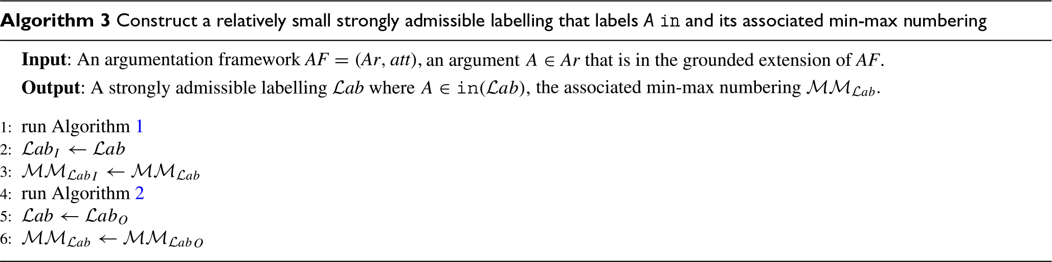
As an example, consider again the argumentation framework of Figure 1. Let C be the main argument. Running Algorithm 1 yields a labelling $(\{A,C,D\},\{B\},\{E,F,H,H\})$ with associated numbering $\{(A:1),(B:2),(C:3),(D:1)\}$ (as explained in Section 3.1). Feeding this labelling and numbering into Algorithm 2 then yields an output labelling $(\{A,C\},\{B\},\{D,E,F,G,H\})$ with associated output numbering $\{(A:1),(B:2),(C:3)\}$ (as explained in Section 3.2).

Given the properties of Algorithm 1 and Algorithm 2, we can prove that Algorithm 3 terminates, correctly computes a strongly admissible labelling and its associated min-max numbering, and runs in polynomial time (more specific, in cubic time).

Theorem 19.

Let $AF=(Ar,att)$ be an argumentation framework and A be an argument in the grounded extension of $AF$ . Let both $AF$ and A be given as input to Algorithm 3. It holds that the algorithm terminates.

Proof.

This follows from Theorem 1 and Theorem 12.

Theorem 20.

Let $AF=(Ar,att)$ be an argumentation framework and let A be an argument in the grounded extension of $AF$ . Let both $AF$ and A be given as input to Algorithm 3. Let $\mathcal{L}ab$ and ${\mathcal{M}\mathcal{M}}_{\mathcal{L}ab}$ be the output of the algorithm. It holds that $\mathcal{L}ab$ is a strongly admissible labelling that labels A $\mathtt{i}\mathtt{n}$ and has ${\mathcal{M}\mathcal{M}}_{\mathcal{L}ab}$ as its min-max numbering.

Proof.

This follows from Theorem 10, Theorem 14, Theorem 16 and Theorem 17.

Theorem 21.

Let $AF=(Ar,att)$ be an argumentation framework and let A be an argument in the grounded extension of $AF$ . Let both $AF$ and A be given as input to Algorithm 3. Let $\mathcal{L}ab$ and ${\mathcal{M}\mathcal{M}}_{\mathcal{L}ab}$ be the output of the algorithm. It holds that Algorithm 3 computes $\mathcal{L}ab$ and ${\mathcal{M}\mathcal{M}}_{\mathcal{L}ab}$ in $O(n^3)$ time.

Proof.

This follows from Theorem 11 and Theorem 18.

Theorem 22.

Let $AF=(Ar,att)$ be an argumentation framework, A be an argument in the grounded extension of $AF$ . Let $AF$ and A be given as input to Algorithm 1 and Algorithm 3. Let $\mathcal{L}{ab}_I$ and ${{\mathcal{M}\mathcal{M}}_{\mathcal{L}ab}}_I$ be the output of Algorithm 1 and let $\mathcal{L}{ab}_3$ and ${{\mathcal{M}\mathcal{M}}_{\mathcal{L}ab}}_3$ be the output of Algorithm 3. It holds that $\mathcal{L}{ab}_3⊑\mathcal{L}a{b}_I$ .

Proof.

This follows from Theorem 13, together with Theorem 10 and the way Algorithm 3 is defined (by successively applying Algorithm 1 and Algorithm 2).

4. Empirical results

Now that the correctness of our algorithms has been proved and their computational complexity has been stated, the next step is to empirically evaluate their performance. For this, we compare both their runtime and output with that of other computational approaches.

4.1. Minimality

Although Algorithm 3 aims to find a relatively small strongly admissible labelling, it is not guaranteed to find an absolute smallest. This is because the problem of finding the absolute smallest admissible labelling is coNP-complete, whereas Algorithm 3 is polynomial (Theorem 21). In essence, we have given up absolute minimality in order to achieve tractability. The question, therefore, is how much we had to compromise on minimality. That is, how does the outcome of Algorithm 3 compare with what would have been an absolute minimal outcome? In order to make the comparison, we apply the ASPARTIX ASP encodings of [11] to determine the absolute minimal strongly admissible labelling.

Apart from comparing the strongly admissible labelling yielded by our algorithm with an absolute minimal strongly admissible labelling, we also compare it with the absolute maximal strongly admissible labelling. That is, we compare it with the grounded labelling. The reason for doing so is that the grounded semantics algorithms (e.g. [12,13]) are to the best of our knowledge currently the only polynomial algorithms for computing a strongly admissible labelling (in particular, for the maximal strongly admissible labelling) that have been stated in the literature. As Algorithm 3 is also polynomial (Theorem 21) this raises the question of how much improvement is made regarding minimality.

For queries, we considered the argumentation frameworks in the benchmark sets of ICCMA’17, ICCMA’19 and ICCMA’21.5 For each of the argumentation frameworks we generated a query argument that is in the grounded extension (provided the grounded extension is not empty). We used the queried argument when one was provided by the competition (for instance, when considering the benchmark examples of the Admbuster class, we took ‘a’ to be the queried argument as this was suggested by the authors of this class). After considering 994 argumentation frameworks, we found that 277 argumentation frameworks yielded a grounded extension that is not empty (meaning they could used for current purposes).

We conducted our experiments on a MacBook Pro 2020 with 8 GB of memory and an Intel Core i5 processor. To run the ASPARTIX system we used clingo v5.6.2. We set a timeout limit of 1000 seconds and a memory limit of 8 GB per query.

For each of the selected benchmark examples, we have assessed the following:

• (1)

  the size of the grounded labelling (determined using the modified version of Algorithm 1 as described in Lemma 9)

  (2)

  the size of the strongly admissible labelling yielded by Algorithm 1

  (3)

  the size of the strongly admissible labelling yielded by Algorithm 3

  (4)

  the size of the absolute minimal strongly admissible labelling (yielded by the approach of [11])

  We start our analysis with comparing the output of Algorithm 1 and Algorithm 3 with the grounded labelling regarding the size of the respective labellings. We found that the size of the strongly admissible labelling yielded by Algorithm 1 tends to be smaller than the size of the grounded labelling. More specifically, the strongly admissible labelling yielded by Algorithm 1 is smaller than the size of the grounded labelling in 63% of the 277 examples we tested for. In the remaining 37% of the examples, their sizes are the same.

  

  Fig. 2.

  The size of output of Algorithm 1 (as a percentage of the grounded labelling).

  Figure 2 provides a more detailed overview of our findings, in the form of a bar graph. The rightmost bar represents the 37% of the cases where the output of Algorithm 1 has the same size as the grounded labelling (that is, where the size of the output of Algorithm 1 is 100% of the size of the grounded labelling). The bars on the left of this are for the cases where the size of the output of Algorithm 1 is less than the size of the grounded labelling. For instance, it was found that in 10% of the examples, the size of output of Algorithm 1 is 80% to 89% of the size of the grounded labelling. On average, we found that the size of the output of Algorithm 1 is 76% of the size of the grounded labelling.

  

  Fig. 3.

  The size of output of Algorithm 3 (as a percentage of the grounded labelling).

  As for Algorithm 3, we found an even bigger improvement in the size of it’s output labelling compared to the grounded labelling. More specifically, the size of the strongly admissible labelling yielded by Algorithm 3 is smaller than the grounded labelling in 88% of the 277 examples we tested for. Figure 3 provides a more detailed overview of our findings in a similar way as we previously did for Algorithm 1. On average, we found that the output of Algorithm 3 has a size that is 25% of the size of the grounded labelling.

  

  Fig. 4.

  The size of output of Algorithm 1 compared to the output Algorithm 3 (as a percentage of the size of the grounded labelling).

  Apart from comparing Algorithm 1 and Algorithm 3 with the grounded labelling, it can also be insightful to compare the two algorithms with each other. In Figure 4, each dot represents one of the 277 examples.6 The horizontal axis represents the size of the output of Algorithm 1, as a percentage of the size of the grounded labelling. The vertical axis represents the size of the output of Algorithm 3 as a percentage of the size of the grounded labelling. For easy reference, we have included a dashed line indicating the situation where the output of Algorithm 1 has the same size as the output of Algorithm 3. Any dots below the dashed line represent the cases where Algorithm 3 outperforms Algorithm 1, in that it yields a smaller strongly admissible labelling. Any dots above the dashed line represents the cases where Algorithm 3 under performs Algorithm 1 in that it yields a bigger strongly admissible labelling. Unsurprisingly, there are no such cases as Theorem 22 states that the output of Algorithm 3 cannot be bigger than the output of Algorithm 1. We found that for 95% of the examples, Algorithm 3 produces a smaller labelling than Algorithm 1. Moreover, we found that on average, the output of Algorithm 3 is 32% smaller than output of Algorithm 1.

  

  Fig. 5.

  The size of output of Algorithm 3 compared to a smallest strongly admissible labelling (as a percentage of the size of the grounded labelling).

  The next question is how the output of our best performing algorithm (Algorithm 3) compares with what would have been the ideal output. That is, we compare the size of the output of Algorithm 3 with the size of a minimal strongly admissible labelling for the main argument, as computed using the ASPARTIX encodings of [11]. The results are shown in Figure 5.

  

  Fig. 6.

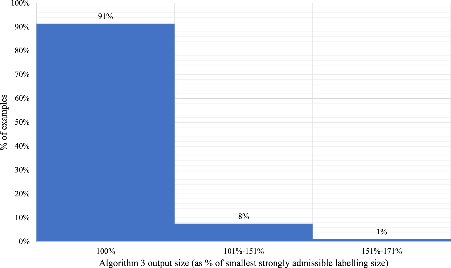
  The size of output of Algorithm 3 compared to a smallest strongly admissible labelling.

  We found that in 91% of the 277 examples, the output of Algorithm 3 is of the same size as the smallest strongly admissible labelling for the output of the main argument. For the other 9% of the examples, the output of Algorithm 3 has a bigger size. On average, we found that the output of Algorithm 3 is 3% bigger than the smallest strongly admissible labelling for the main argument. Figure 6, provides a more detailed overview of how much bigger the output of Algorithm 3 is compared to the smallest strongly admissible labelling for the main argument.

  4.2. Runtime

  The next thing to study is how the runtime of our algorithms compares with the runtime of some of the existing computational approaches. In particular, we compare the runtime of Algorithm 1 and Algorithm 3 with the runtime of the ASPARTIX-based approach of [11].

  
  Fig. 7.

  The runtime of Algorithm 3 compared to the runtime of computing the grounded labelling using Algorithm 3 of [13].

  We first compare the runtime of Algorithm 3 to the runtime of the modified version of Algorithm 3 of [13] for computing the grounded labelling. It turns out that the runtimes of these algorithms are very similar. On average, Algorithm 3 of [13] took 0.02 seconds (3%) more than Algorithm 3 to solve the test instances. These runtime results of Algorithm 3 and Algorithm 3 of [13] are shown in Figure 7.

  
  Fig. 8.

  The runtime of computing a smallest admissible labelling using the ASPARTIX encodings compared with the runtime of Algorithm 3.

  The next question is how does the runtime of computing Algorithm 3 compare to the runtime of the ASPARTIX encoding for minimal strongly admissibility. It was observed that the runtime of ASPARTIX encoding is significantly longer than the runtime of Algorithm 3. A detailed overview of the difference in runtimes of Algorithm 3 and the ASPARTIX encoding on minimal strong admissibility is shown in Figure 8. On average, the ASPARTIX framework took 12.5 seconds (907%) more than Algorithm 3 to solve the test instances.

5. Discussion

In the current paper, we provided two algorithms (Algorithm 1 and Algorithm 3) for computing a relatively small strongly admissible labelling for an argument that is in the grounded extension. We proved that both algorithms are correct in the sense that each of them returns a strongly admissible labelling (with associated min-max numbering) that labels the main argument $\mathtt{i}\mathtt{n}$ (Theorem 10 and 20). Moreover, each algorithm runs in polynomial (cubic) time (Theorem 11 and Theorem 21). It was also shown that the strongly admissible labelling yielded by Algorithm 3 is smaller than or equal to the strongly admissible labelling yielded by Algorithm 1 (Theorem 13).

The next question we examined is how small the output of Algorithm 1 and Algorithm 3 is compared to the smallest strongly admissible for the main argument. Unfortunately, previous findings make it difficult to provide formal theoretical results on this. This is because the c-approximation problem for strong admissibility is NP-hard, meaning that a polynomial algorithm (such as Algorithm 1 and Algorithm 3) cannot provide any guarantees of yielding a result within a fixed parameter c from the size of the absolute smallest strongly admissible labelling for the main argument.

Hence, instead of developing theoretical results, we decided to approach the issue of minimality in an empirical way, using a number of experiments. These experiments were based on the benchmark examples that were submitted to ICCMA’17, ICCMA’19 and ICCMA’21. We compared the output of Algorithm 1 and Algorithm 3 with both the biggest and the smallest strongly admissible set for the main argument (the biggest was computed using Algorithm 3 described in [13] and the smallest was computed using the ASPARTIX based approach on computing minimal strong admissibility in [11]). Overall, we found that Algorithm 3 yields results that are only marginally bigger than the smallest strongly admissible labelling, with a run-time that is a fraction of the time that would be required to find this smallest strongly admissible labelling. The outputs of both algorithms return a strongly admissible labelling that is significantly smaller than the biggest strongly admissible labelling (the grounded labelling), with the output of Algorithm 3 on average being only 25% of the size of the biggest strongly admissible labelling.

Although our Algorithm 3 tends to yield good results in most cases (obtaining an absolute smallest strongly admissible labelling in 91% of the examples we tested for) there are some argumentation frameworks where it will not perform well. An example of such an argumentation framework is shown in Figure 9.

Fig. 9.

An example of an argumentation framework where Algorithm 3 yields a strongly admissible labelling that is not minimal.

For the argumentation framework of Figure 9, Algorithm 3 will yield the strongly admissible labelling $(\{A,H,J,L,N\},\{B,I,K,M\},\{C,D,E,F,G\})$ with associated min-max numbering $\{(A:5),(B:4),(H:3),(I:2),(K:2),(M:2),(J:1),(L:1),(N:1)\}$ . However, this labelling is not minimal, as the minimal strongly admissible labelling is $(\{A,C,E,G\},\{B,D,F\},\{H,I,J,K,L,M,N\})$ with associated min-max numbering $\{(A:7),(B:6),(C:5),(D:4),(E:3),(F:2),(G:1)\}$ .

To understand how such a suboptimal result was produced, it is important to realise that Algoritm 2, when choosing an $\mathtt{i}\mathtt{n}$ -labelled attacker of an $\mathtt{o}\mathtt{u}\mathtt{t}$ -labelled argument (e.g. Algorithm 2 arriving at argument B and having to choose between C and H) makes this choice based on which of those attackers have the smallest min-max number (line 19 of Algorithm 2). In the case of the argumentation framework of Figure 9, Algorithm 2 will choose H instead of C, even though C would have been a better choice. This is because even though the branch starting with C is longer, it does not have the same fan-out as the branch starting with H, resulting in fewer arguments that need to be labelled $\mathtt{i}\mathtt{n}$ and $\mathtt{o}\mathtt{u}\mathtt{t}$ . In general, the heuristic of choosing the attacker with the smallest min-max number can be suboptimal,7 especially for argumentation frameworks where shorter branches tend to have a higher fan-out. It is likely to still perform quite reasonable when the fan-out is spread more or less equally among branches of different length. The fact that our Algorithm 3 manages to yield an absolute smallest strongly admissible labelling in 91% of cases, based on the ICCMA’17, ICCMA’19 and ICCMA’21 benchmark sets, indicates that the kind of argumentation frameworks where our algorithm performs poorly are perhaps not very common.

Algorithm 1 requires that the main argument (argument A) is in the grounded extension. At first sight, this would seem to require some additional computation before our algorithms are run, in order to determine whether this is indeed the case. However, it would not be difficult to modify Algorithm 1 to provide an answer to this as well.8 This could be done by not only returning a labelling and its associated min-max numbering, but by also returning a flag that indicates whether argument A is actually part of the grounded extension. This flag would be set to true if $\mathcal{L}ab$ and ${\mathcal{M}\mathcal{M}}_{\mathcal{L}ab}$ are returned at line 16 or line 33. The idea is to return false if the algorithm reaches line 39 (instead of printing an error message). In the latter case, one could additionally return $\mathcal{L}ab$ and ${\mathcal{M}\mathcal{M}}_{\mathcal{L}ab}$ , which would be the grounded labelling and its associated min-max numbering (the proof of this would be similar to that of Lemma 9). This grounded labelling and associated min-max numbering would provide evidence that argument A is not part of the grounded extension. It can easily be verified that Theorem 1 as well as Lemma 2, 3, 4, 5, 6, 7 still hold in such a case, as none of these depend on argument A being in the grounded extension. Moreover, the complexity of the algorithm would remain cubic.

Algorithm 2 could to some extent be optimised by adding an extra condition to line 15, so that the for-loop only runs for attackers that are not yet labelled $\mathtt{o}\mathtt{u}\mathtt{t}$ .9 Without such a condition, lines 16 and 17 could run unnecessary, as the two assignments may already have been done previously. However, in such a case the if-statement of line 18 will never have its condition fulfilled, hence putting a limit in the advantages of implementing the extra condition in line 15.

The research of the current paper fits into our long-term research agenda of using argumentation theory to provide explainable formal inference. In our view, it is not enough for a knowledge-based system to simply provide an answer regarding what to do or what to believe. There should also be a way for this answer to be explained. One way of doing so is by means of (formal) discussion. Here, the idea is that the knowledge-based system should provide the argument that is at the basis of its advice. The user is then allowed to raise objections (counterarguments) which the system then replies to (using counter-counter-arguments), etc. In general, we would like such a discussion to be (1) sound and complete for the underlying argumentation semantics, (2) not be unnecessarily long, and (3) be close enough to human discussion to be perceived as natural and convincing

As for point (1), sound and complete discussion games have been identified for grounded, preferred, stable and ideal semantics [4]. As for point (2), this is what we studied in the current paper, as well as in [3,6]. As for point (3), this is something that we are aiming to report on in future work.

For future research, it is possible to conduct a similar sort of analysis (as in this paper) on minimal admissible labellings. It was reported obtaining an absolute minimal admissible labelling for a main argument is also of coNP-complete complexity [3,6] therefore, it would be interesting to look into developing an algorithm that generates a small admissible labelling in polynomial time complexity. Similarly, it would also be interesting to look at the complexity and empirical results on generating minimal ideal sets.