Sage Journals: Discover world-class research

Abstract

Many practical tasks in robotic systems, such as cleaning windows, writing, or grasping, are inherently constrained. Learning policies subject to constraints is a challenging problem. In this paper, we propose a method of constraint-aware learning that solves the policy learning problem using redundant robots that execute a policy that is acting in the null space of a constraint. In particular, we are interested in generalizing learned null-space policies across constraints that were not known during the training. We split the combined problem of learning constraints and policies into two: first estimating the constraint, and then estimating a null-space policy using the remaining degrees of freedom. For a linear parametrization, we provide a closed-form solution of the problem. We also define a metric for comparing the similarity of estimated constraints, which is useful to pre-process the trajectories recorded in the demonstrations. We have validated our method by learning a wiping task from human demonstration on flat surfaces and reproducing it on an unknown curved surface using a force- or torque-based controller to achieve tool alignment. We show that, despite the differences between the training and validation scenarios, we learn a policy that still provides the desired wiping motion.

Keywords

Direct policy learning constrained motion null-space policy force/torque application

1. Introduction

When performing a given task in an unfamiliar environment, human beings easily adapt the skills or previously learned motions to novel situations and environments. For instance, the operator in Figure 1 wipes the front panels of the train by employing a small set of motions and skills that generalize to different train geometries and positioning (Moura and Erden, 2017). However, current robotic systems often require computationally expensive replanning and precise scans of the new environment to reproduce a given task (Pastor et al., 2011; Shiller, 2015). In addition to this, movement in complex, high degree of freedom manipulation systems often contains a high level of redundancy. The degrees of freedom available to perform a task are usually higher than what is necessary to execute that task. This allows a certain flexibility in finding an appropriate solution, so that this redundancy may be resolved according to some strategy that achieves a secondary objective, while the primary task is not affected. Such approaches to redundancy resolution are employed by human beings (Cruse and Brüwer, 1987), as well as other redundant systems, such as (humanoid) robots (D’Souza et al., 2001).

Fig. 1.

Manual cleaning of an electric train. Willesden depot, London (2016).

The redundancy resolution may also be interpreted as a form of hierarchical task decomposition, in which the complete space of available movement is split into a task-space component and a null-space component. For instance, one might consider a primary task, such as reaching or trajectory tracking, and a lower-priority task as a secondary goal, such as avoiding joint limits (Gienger et al., 2005), self-collisions (Sugiura et al., 2006), or kinematic singularities (Yoshikawa, 1985). This notion is particularly evident when considering motions modulated by external or environmental constraints. For instance, in the wiping task of Figure 1, the tool is constrained by the window surface; the primary task is to keep the tool aligned and in contact, and the secondary task is to provide surface coverage while maintaining a comfortable arm position. Several variants of this hierarchical approach to redundancy have been used in robotics (Khatib et al., 2008). This core concept has been applied to task sequencing (Mansard and Chaumette, 2007), task prioritization (Baerlocher and Boulic, 2004), and hierarchical quadratic programming (Escande et al., 2014; Herzog et al., 2015). These methods minimize a cost function subject to known constraints. However, they suffer from the curse of dimensionality and are typically unsuitable for real-time applications in high dimensions.

To circumvent this problem, one might attempt to learn a policy, a mapping from states to actions, that encodes behavior consistent with the set of constraints, instead of continuously calculating constraint-consistent actions. This mapping can be learned from data captured during demonstrations, consisting of human or robot motions. This approach falls under the category of imitation learning or learning by demonstration (Argall et al., 2009). One straightforward way to learn behaviors from this is through direct policy learning (DPL) (Alissandrakis et al., 2007; Calinon and Billard, 2007; Schaal et al., 2003). For instance, Gams et al. (2014) proposes to use a modification of dynamic movement primitives (Ijspeert et al., 2003) so that limits are considered at velocity and acceleration levels to tune the interaction forces of a robotic system with an object. Although DPL is well known and widely used, other approaches related to the problem of learning by demonstration involve learning a “filtered” trajectory over the demonstrations and combine operational and configuration tasks within a probabilistic framework. In particular, Calinon (2016) and Hussein et al. (2015) propose to use a Gaussian mixture model or Gaussian mixture regression to learn a parametrized trajectory with known tasks constraints, while Paraschos et al. (2017) propose that learning the prioritization of tasks can also enable the estimation of “soft” constraints and a prioritization between them.

In this paper, the problem of learning by demonstration will be understood as an action mapping in a DPL context (Alissandrakis et al., 2007; Schaal et al., 2003); however, it is well known that this method suffers from poor generalization (Argall et al., 2009) under varying unknown constraints. On the contrary, constraint-aware learning, in which the task or constraint is learned first and a null-space policy common to all tasks is learned separately using conventional methods has been shown to provide significant improvements (Armesto et al., 2017a,b; Lin et al., 2015; Towell et al., 2010). The idea behind constraint-aware methods is that the raw input data can be projected onto the null space of the task or constraint once it has been learned. We can then use other learning methods for the unconstrained policy, which is assumed to be the same across all demonstrations (Lin et al., 2015). Such an approach falls under the categorization of “hard” constraint methods (Paraschos et al., 2017). Lin et al. (2015). Lin et al. (2015) present a method for estimating the null-space projection matrix. The main drawback of their approach is that the estimation is performed by solving a non-convex optimization problem using a spherical representation. This often leads to long computation times and decreased performance (Armesto et al., 2017a). In this paper, we present a closed-form solution of this problem.

The results presented in this paper are, indeed, an extension of (Armesto et al., 2017b), in which we provide a more detailed explanation and justification of the proposed method. In particular, we consider a DPL problem, which might be difficult to learn, by making a reasonable separation into two subproblems: learning the constraint and learning the null-space policy, where both subproblems have closed-form solutions with linear parametrization. This improvement allows us to estimate null-space projection matrixes from data of different tasks, which can be used for learning a null-space policy by observing multiple projections of such a policy. Howard and Vijayakumar (2007) later use this estimate to learn the null-space policy. One of the key differences between our approach and that presented by Lin et al. (2015) is that in this paper we propose learning the constraint equation by minimizing the error in the task-space, while Lin et al. (2015) perform the minimization on an error defined in the null space. Secondly, Lin et al. (2015) impose the assumption of having access to the null space, while here we can deal with data containing both task and null-space components. In addition to this, we split the raw observation into task and null-space components in a more efficient way than the method proposed by Towell et al. (2010). Lin et al. (2017) also efficiently split the learning method into task and null-space components, but for lower-dimensional systems, unlike our method. To estimate the null-space policy, we propose to use locally weighted models (Atkeson et al., 1997); however, the method used to model such a policy is not that relevant and other well-known approaches in DPL might also be used (Calinon, 2016; Hussein et al., 2015; Ijspeert et al., 2003). We show that the learned policy can then be executed online by using a force-sensor-based task to align to an arbitrary surface.

The contributions of this paper are:

We formulate the constrained learning problem as a joint optimization over both constraint and policy parameters. Since this is a difficult problem to solve in practice, we then propose an alternate formulation, which splits this optimization into two subproblems, which we solve sequentially.

We formulate a closed-form solution of these subproblems by making them linear in their respective parameters.

We extend the theoretical work of hierarchically constrained optimization presented by Escande et al. (2014) and adapt it for the domain of constraint-aware learning from demonstration.

We develop a metric for computing the similarity of estimated constraints.

We show that our framework can employ generic models to represent the constraints and policies with no prior knowledge. We then show how application-specific knowledge can be exploited by using domain-specific regressors with physical meaning.

We validate our method through experiments by learning a circular wiping policy from human demonstrations on planar surfaces.

We define a surface alignment task using a force sensor, allowing us to perform wiping on curved surfaces based on the previously learned policy.

2. Preliminaries and problem statement

In many robotics applications, we can decompose the motion policy into a hierarchy of sub-policies. For instance, in such applications as welding, ironing, wiping, writing, etc., we can split the overall policy into a primary task of maintaining the contact with the working surface, and a secondary task of tracing a specific trajectory along the surface. Additionally, we might even specify a third task of avoiding joint limits, or minimizing deviations from a comfortable pose. In this case, a task from a higher level in the hierarchy acts as a constraint on the lower-level policies. In learning from demonstration, we assume that we have been given demonstrations of the kind of motion that we want to describe by a mathematical model.

Let us assume a system with control input $u (t) \in ℝ^{q}$ , which is subject to the following Pfaffian constraint

$A (t) u (t) = b (t)$ (1)

where $A (t) \in ℝ^{s \times q}$ is a full row-rank Pfaffian constraint matrix and $b (t) \in ℝ^{s}$ is denoted as the primary-task policy. When $s < q$ , there exists a null-space policy $π (t) \in ℝ^{q}$ , such that the control action in equation (1) can be obtained as

$u (t) = A {(t)}^{†} b (t) + N (t) π (t)$ (2)

where $N (t) : = I - A {(t)}^{†} A (t)$ is a projection matrix of the right null space of $A (t)$ and † denotes the Moore–Penrose pseudoinverse. The control action can be divided into task ${}^{ts}u (t)$ and null-space components ${}^{ns}u (t)$

$\begin{matrix} {}^{ts}u (t) : = A {(t)}^{†} b (t) \end{matrix}$ (3)

$\begin{matrix} {}^{ns}u (t) : = N (t) π (t) \end{matrix}$ (4)

Note that, by definition, ${}^{ts}u (t) ⊥^{ns} u (t)$ , and the primary-task ( $b (t)$ ) and null-space ( $π (t)$ ) policies form the full control action. Actually, as $N (t) A {(t)}^{†} = 0$ and $N {(t)}^{2} = N (t)$ , from equation (2) we can assert that

${}^{ns}u (t) = N (t) u (t)$ (5)

In a DPL context, an action mapping involves searching for optimal parameters $w_{u}$ (Schaal et al., 2003; Alissandrakis et al., 2007)

$w_{u}^{*} : = \underset{w_{u}}{argmin} ∥ u (t) - U (w_{u}, t) ∥^{2}$ (6)

where the norm is defined, given $α : [0, T] \mapsto ℝ^{n}$ , as

$∥ α (t) ∥ : = \sqrt{\frac{1}{T} \int_{0}^{T} α^{⊤} (t) α (t) dt}$

and $U (w_{u}, t)$ is a suitably parametrized function approximator, with $w_{u}$ the adjustable parameters, i.e. parameters from a policy model $U (w_{u}, t)$ , which could be solved using any optimization procedure. In most cases, choosing a linear-in-parameter approximator will allow computationally simpler learning algorithms to be employed, as discussed later on.

Calinon and Billard (2007) proposed to solve this problem using a method they called DPL. This is a special case of our formulation that ignores the task hierarchy, pursuing a direct optimization of equation (6).

However, such a direct approach cannot “distinguish” between the actions needed to achieve the primary task (constraint satisfaction) and the actions needed to carry out the secondary task (for instance, tracing a trajectory in the constraint space). Furthermore, the primary task can often be achieved using inverse kinematics or reactively using force or visual feedback. This shifts the focus onto learning a policy that is aware of the acting constraint imposed by the primary task. This idea is implicit in the separation into task-space and null-space components in equations (3) and (4). The inability of DPL to separate such components in the learning process motivates the main goal of this paper: setting up a suitable parametrization and formulating an optimization problem such that the aforementioned constraint-aware learning is possible.

In a generic scenario, the problem is solved using a training dataset with samples of states and controls. However, the dataset might contain data coming from a mixture of different constraints, tasks, and policies. Our problem statement encompasses all these possible situations if the dataset is extended by encoding the different constraints and tasks onto pieces of time-varying information. This additional information classifies the training dataset according to the relevant task or constraint information, to produce an estimate of the null-space policy $π (t)$ consistent with such classification. Obviously, in a specific implementation, this idea may require the data to be annotated using a set of subindices referring to a specific constraint, task, or demonstration. However, with no loss of generality, we omit such indexing to avoid cluttering the notation until it is required for the implementation in the example sections. If such training data classification is not known, it might be inferred directly from the data, as shown in the last example of this paper.

3. Constraint-aware policy learning

When learning the policy $π (t)$ from constrained data, we assume that matrixes $A (t)$ , $b (t)$ , and $N (t)$ are not known. However, they will be given or estimated from sensor data when executing the learned policy, i.e. estimating surface parameters using computer vision and aligning the end effector with the surface. This is useful, because the learned policy can be projected onto the estimated constraint.

Given this assumption, the aim is to learn a null-space policy $π (t)$ from constrained data for a given set of demonstrations, so that they can be reproduced under different constraints in real operation using sensor-based data. In that sense, for a given $u (t)$ , we want to estimate the constraint matrix $A (t)$ and task $b (t)$ . Later on, by combining data from all demonstrations, we will learn $π (t)$ .

Learning is usually carried out by parametrized approximators, which are continuous functions. For instance, universal function approximators, such as the ones proposed by Hornik et al. (1989) provide progressively more accurate approximations as the number of parameters, neurons, etc., increases. Let us assume that the set of constraint matrix, task, and null-space policy can be parametrized as

$\begin{matrix} A (t) : = A (w, t) \end{matrix}$ (7)

$\begin{matrix} b (t) : = b (w, t) \end{matrix}$ (8)

$\begin{matrix} π (t) : = π (w, w_{π}, t) \end{matrix}$ (9)

where we can consider the parameters of the DPL problem in equation (6) to be $w_{u} : = (w, w_{π})$ in equations (7) to (9).

Note that the actual explicit expression of equations (7) to (9) would depend on some problem-dependent information available at time t. In most cases, this will be the robot state, but there might also be other task or constraint-dependent information, as discussed in the previous section. For instance, from the robot’s forward kinematics, expressed as $f (x (t), w, t) = 0$ , the Pfaffian constraint is derived as

$A (x (t), w, t) : = \frac{\partial f}{\partial x (t)} (x (t), w, t)$

and

$b (x (t), w, t) : = \frac{\partial f}{∂t} (x (t), w, t)$

with $u (t) \equiv \dot{x} (t)$ . If $f$ is time-invariant (no explicit dependence on t), then $b (t) \equiv 0$ . This particular case is, indeed, common in many situations, if we assume that the demonstration trajectories lie on a fixed “surface”.

From this task or null-space parametrization, given a set of demonstrations, the DPL can be reformulated as the “constraint-aware policy learning” (CAPL) problem of minimizing equation (6) with the parametrization

$U (w_{u}, t) : = A {(w, t)}^{†} b (w, t) + N (w, t) π (w, w_{π}, t)$ (10)

i.e., minimizing

$\begin{matrix} J (w_{u}) : = \\ {∥u (t) - A {(w, t)}^{†} b (w, t) - N (w, t) π (w, w_{π}, t)∥}^{2} \end{matrix}$ (11)

Of course, the DPL cost (equation (6)) may be directly optimized with a suitable parametrization. However, the assumption that the demonstrations are provided under the previously discussed constraints suggests that equation (10) might be a better parametrization than a generic “constraint-unaware” parametrization of $U$ . For instance, if we consider a state-dependent policy, $U (x, w_{u})$ , a set of training demonstrations might have different actions for the same state under different constraints (data inconsistency); see the example in Section 6.1, where intersecting circles in different orientations illustrate such a case. In this situation, constraint-unaware DPL would try to “average” the actions for a state, whereas the constraint-aware learning method would involve correctly learning a different action for each constraint; see the details in Section 6.1.

In practice, this problem is difficult to solve because, even if the approximators (equation (7) to (9)) were linear in their parameters, the presence of pseudoinverses in equation (11) introduces a complex relation with respect to $w$ . However, under mild assumptions, we can reasonably approximate the original cost function by splitting it into two simpler optimization problems. Indeed, we recall that, for any orthogonal matrix $Ω$ , we have $∥ e ∥ = ∥ Ω e ∥$ . This will inspire an orthogonal change of coordinates, yielding a factored expression of $J (w_{u})$ but keeping the same optimal parameter values.

Lemma 1. If rows of $A (w, t)$ are orthonormal, i.e., if $A (w, t)$ is a semi-orthogonal matrix,¹ then we can express equation (11) as

$J (w, w_{π}) = J_{1} (w) + J_{2} (w, w_{π})$ (12)

where

$\begin{matrix} J_{1} (w) : = {∥A (w, t) u (t) - b (w, t)∥}^{2} \end{matrix}$ (13)

$\begin{matrix} J_{2} (w, w_{π}) : = {∥N (w, t) (u (t) - π (w, w_{π}, t))∥}^{2} \end{matrix}$ (14)

The proof of this lemma can be found in Appendix A.

3.1. Sequential optimization

We can approximately solve the constraint-parametrized learning problem sequentially, first minimizing $J_{1} (w)$ by searching for optimal parameters $w^{*}$ and then fixing these parameters while minimizing $J_{2} (w^{*}, w_{π})$ over $w_{π}$ . The approximation comes from the fact that $w$ and $w_{π}$ are computed in sequence, even though J₂ also depends on $w$ . Thus, if the solution of the sequential minimization makes both J₁ and J₂ small (say, compared with $∥ u (t) ∥$ ), then we have a good solution for the original J. However, if the value of J₂ were large, a joint optimization of equation (11) might obtain better results (albeit with the mentioned computational drawbacks). Nevertheless, this might also indicate that richer functions approximations are needed; this would certainly be the case if $J_{1} (w^{*})$ were large as, evidently, the optimal value of J will be always larger than $J_{1} (w^{*})$ , since $J_{2} \geq 0$ .

The advantage of this approach is that $J_{2} (w^{*}, w_{π})$ can be minimized using the standard least-squares method if we use a linear parametrization of $π (w, w_{π})$ with respect to $w_{π}$ . Additionally, regarding $J_{1} (w)$ , parameters $w^{*}$ can be computed in closed form using a generalized eigenvalue method, as we will show now.

3.2. Closed-form constraint estimation

In this section, we define a method for solving the minimization of equation (13). Hence, it will allow us to estimate the constraint matrix and the associated null-space projection matrix, which will be used to split the action observations into task-space and null-space components.

Note that equation (13) only depends on parameters $w$ . We can compute these parameters from the demonstrated data. If we express $A (w, t)$ and $b (w, t)$ as a linear combination of regressors,² they could be defined, at any time, as

$\begin{matrix} A (w, t) : = w_{A} Φ_{A} (t) \end{matrix}$ (15)

$\begin{matrix} b (w, t) : = w_{b} Φ_{b} (t) \end{matrix}$ (16)

where $w_{A} \in ℝ^{s \times w_{A}}$ and $w_{b} \in ℝ^{s \times w_{b}}$ are constant matrixes composed of parameters to be learned, $w : = (w_{A}, w_{b})$ . $Φ_{A} (t) \in ℝ^{w_{A} \times n}$ , and $Φ_{b} (t) \in ℝ^{w_{b}}$ are some regressors that can be evaluated from information of the demonstrated motion at time t, e.g. the state $x (t)$ , the end-effector position computed from this state, or any other arbitrary function. This information may, for instance, describe some task information, as we discuss later.

Let us, for convenience, define

$\begin{matrix} Δ (w, t) = A (w, t) u (t) - b (w, t) \\ = [w_{A} w_{b}] [\begin{matrix} Φ_{A} (t) u (t) \\ - Φ_{b} (t) \end{matrix}] \\ = w H (t) \end{matrix}$ (17)

where $H (t)$ comprises all the regressors (multiplied by the control inputs in the case of those from $A (w, t)$ ) into a single matrix.

We now want to compute the parameters $w^{*}$ that will fit the regressors to the demonstrated data using a least-squares technique. The solution can be computed via the generalized eigenvalues and eigenvectors, as described in Lemma 2.

Lemma 2. Consider the problem of minimizing $J : = θ^{⊤} R θ$ subject to $θ^{⊤} Q θ = 1$ , with $R$ and $Q$ symmetric. The optimal value of J is $λ$ , where $λ$ is the minimum generalized eigenvalue of the linear matrix pencil $λ Q - R$ . The minimizer $θ$ must be a generalized eigenvector corresponding to eigenvalue $λ$ .

The proof of this lemma appears in Appendix B.

Now, recall that a “demonstration” will be a set of controls at different time instants from, say $t = 0$ to $t = T$ . Thus, the (Euclidean) norm in $J_{1} (w)$ will actually be expressed as

$w (\int_{0}^{T} H (t) H^{⊤} (t) dt) w^{⊤}$ (18)

subject to

$1 = w [\begin{matrix} Φ_{A} (t) Φ_{A} {(t)}^{⊤} & 0 \\ 0 & 0 \end{matrix}] w^{⊤} \forall t \in [0, T]$ (19)

However, depending on the chosen parametrization, this constraint might be difficult to satisfy. Therefore, we propose to approximate $J_{1} (w)$ with an average unit-norm constraint, i.e., enforcing

$w [\begin{matrix} \frac{1}{T} \int_{0}^{T} Φ_{A} (t) Φ_{A} {(t)}^{⊤} dt & 0 \\ 0 & 0 \end{matrix}] w^{⊤} = 1$ (20)

Now, applying Lemma 2, we can obtain the optimal values for $w$ by minimizing equation (18) subject to the constraint (equation (20)). To do this, we compute $R = \int_{0}^{T} H (t) H^{⊤} (t) dt$ from equation (18) and a rank-deficient $Q$ from equation (20).

Note that, in practice, these integrals would be evaluated via a sum of the available data samples, i.e., if we have N uniformly sampled data points, we can arrange the $H$ matrix as

$H : = [\begin{matrix} Φ_{A} (t_{1}) u (t_{1}) & Φ_{A} (t_{2}) u (t_{2}) & \dots & Φ_{A} (t_{N}) u (t_{N}) \\ Φ_{b} (t_{1}) & Φ_{b} (t_{2}) & \dots & Φ_{b} (t_{N}) \end{matrix}]$ (21)

where $u (t_{1}), u (t_{2}), \dots, u (t_{N})$ are the raw observations of the action from the demonstration, with $t_{1} = 0$ , $t_{N} = T$ . Then, the integral in equation (18) would be evaluated as $\frac{1}{N} H H^{⊤}$ and an analogous approach would be taken for equation (20).

In theory, if several constraints are fulfilled with no error, then the (generalized) eigenvalue zero would have a multi-dimensional subspace of eigenvectors; thus, an orthogonal basis of such eigenvectors would form the rows of $w_{A}$ and $w_{b}$ . However, in practice, such a situation might not occur with noisy demonstrations so the smaller eigenvalues should be interpreted as being zero. This is a common practice in the “total-least-squares” and “principal-components” techniques discussed in Zhang (2017), to which this proposal is related.

Note that, in this noisy case, the overall result of this first phase of the learning methodology is a matrix $w^{*}$ of parameters associated to low eigenvalues, which fulfills $A (x (t), w^{*}, t) u (t) \approx b (x (t), w^{*}, t)$ . Once the parameters have been learned, we can compute a modified task vector $\tilde{b} (t) : = A (x, w^{*}, t) u (t)$ such that the Pfaffian constraint is fulfilled exactly.

If $b (t) = 0$ , it can be shown (details omitted for brevity) that the problem reduces to removing the rows of $H$ related to $Φ_{b}$ in equation (21), and computing the smallest singular values or vectors of $ϒ^{- 1} H$ , where $ϒ$ is a scaling matrix, such that

$ϒ ϒ^{⊤} : = \frac{1}{T} \int_{0}^{T} Φ_{A} (t) Φ_{A} {(t)}^{⊤} dt$

generalizing the work of Armesto et al. (2017b). Actually, if the number of constraints is known in advance, it is easy to discriminate between situations where there is an over- or under-parametrization by computing the number of significantly smaller eigenvalues. Thus, if the number of significant eigenvalues is smaller than the expected number of constraints, it implies that there is an under-parametrization and more regressors should be added. On the contrary, if the number of significantly smaller eigenvalues is greater than the number of expected constraints, either the problem is over-parametrized or the data fulfill more constraints than originally assumed.

3.3. Learning the null-space policy

At this stage, once the minimization of $J_{1} (w)$ has been carried out and $w^{*}$ is available, each data point in the dataset can be split into its null-space and task-space components, as

$\begin{matrix} {}^{ns}u (w^{*}, t) : = N (w^{*}, t) u (t) \end{matrix}$ (22)

$\begin{matrix} {}^{ts}u (w^{*}, t) : = u (t) - {}^{ns}u (w^{*}, t) \end{matrix}$ (23)

This can be interpreted as an estimate of the “true” null-space and task-space components (equations (3) and (4)), if the relevant eigenvalues are close to zero. Note also that $A {(w^{*}, t)}^{ns} u (w^{*}, t) = 0$ and $A {(w^{*}, t)}^{ts} u (w^{*}, t) = \tilde{b} (t)$ .

Now, we can estimate the optimal value of $w_{π}$ from equation (14) evaluated at $w^{*}$

$J_{2} (w^{*}, w_{π}) = {∥{}^{ns}u (w^{*}, t) - N (w^{*}, t) π (w^{*}, w_{π}, t)∥}^{2}$ (24)

Since $π (w^{*}, w_{π}, t)$ is linear in parameters $w_{π}$ , this corresponds to a standard least-squares problem.

3.4. Learning with locally weighted models

There are several ways in which we can model the policy $π (w^{*}, w_{π}, t)$ . Let us consider a very generic state-feedback policy $π (x (t), w_{π}, t)$ . This simple model has also been adopted by Howard et al. (2009), Lin et al. (2015), and Towell et al. (2010). Indeed, the robot configuration $x (t)$ will often encode essential features of the constraint. For instance, if we assume that all demonstrations keep a constant orientation of the end effector with respect to the normal vector of the constraint surface, then the normal of the surface will be represented in some features of the robot’s state (we exploit this particular constraint later in this paper). We can implicitly replace dependence on $w^{*}$ with the dependence on $x (t)$ in applications where closed-loop feedback in the primary task will ensure that the position or orientation constraints are maintained during real-time operation.

Based on this idea, $π (x (t), w_{π}, t)$ will be defined as a weighted combination of M local models, as

$π (x (t), w_{π}, t) : = \frac{\sum_{m = 1}^{M} ρ_{m} (x (t)) π_{m} (x (t), w_{π, m}, t)}{\sum_{m = 1}^{M} ρ_{m} (x (t))}$ (25)

where each local model m is parametrized by a corresponding $w_{π, m}$ with $w_{π} : = (w_{π, 1}, \dots, w_{π, M})$ , and $ρ_{m} (x (t)) : = e^{- \frac{1}{2} {(x (t) - c_{m})}^{⊤} D_{m}^{- 1} (x (t) - c_{m})}$ is the importance weight of each state observation according to the distance from a Gaussian receptive field, with center $c_{m}$ and variance $D_{m}$ (a diagonal matrix). The centers and variances of the receptive fields can be obtained from data, for instance, by running the k -means algorithm presented by Kanungo et al. (2002).

For each local model, we use a regressor vector $Ψ (x (t), t)$ with linear parameters, as

$π_{m} (x (t), w_{π, m}, t) : = Ψ (x (t), t) w_{π, m}$ (26)

where $w_{π, m}$ , for $m = 1, \dots, M$ are the weight vectors to be learned. If the receptive fields $ρ_{m} (x (t))$ are dense enough and the constraint is time-independent, the local regressors $Ψ (x (t), t)$ may be chosen as simple linear functions $Ψ (x (t), t) : = [x {(t)}^{⊤} 1]$ . Indeed, the nonlinearity will be handled by mixing local linear models, as studied by Atkeson et al. (1997). The described regressor choice can now be inserted into equation (24) to form the associated least-squares problem. In a more general case, we would consider a policy $π (x (t), w, w_{π}, t)$ that depends on the parameters of the primary task. The regressors may then also depend on these parameters $Ψ (x (t), w^{*}, t)$ .

Actually, note that the local-model structure can, too, be used to form the regressors for $A (x (t), w, t)$ and $b (x (t), w, t)$ , which could model a nonlinear constraint in the same way.

If we have prior information about the policy we are attempting to learn, we can choose specific regressors if we believe that they will represent the task better. This may improve accuracy and reduce the number of parameters, compared with other options. For instance, a task involving tracing end-effector trajectories may use the rows of the end-effector Jacobian as regressors. The choice of suitable regressors is application-dependent. In our case study, we discuss the selection of regressors suitable for learning policies that are constrained to a planar surface.

4. Learning planar-constrained policies

Defining the appropriate set of regressors can be difficult without prior knowledge about the application. In this section, we propose to exploit the prior knowledge of the application by using Jacobians of the end effector as the main regressors for learning both the constraint and the null-space policy. This will allow us to define exact models for tasks demonstrated on planar surfaces. However, once the model has been trained, the policy can be executed on non-planar surfaces as long as we can guarantee that the end effector will stay aligned with the surface (e.g. by using force feedback). This parametrization is useful for applications where the robot is constrained by a surface on which the task is being performed, such as wiping, dusting, sweeping, scratching, or writing. In all these examples, a constraint could be defined in terms of minimizing the distance from the surface and the misalignment between the surface normal and the orientation of the robot’s tool (see Figure 2). The null space of this task would be any motion of the robot’s tool on the surface, i.e., with speed of movements tangential to the surface.

Fig. 2.

Robot performing constrained task on curved surface. The robot uses a force sensor and a soft material (sponge) mounted at the end effector as a tool. The interaction of the wiping tool and the surface causes a friction force $f_{f}$ , a normal force $f_{n}$ , and a contact torque $m_{c}$ , where the arrows indicate the direction in which the values $f_{x}$ and $f_{z}$ are measured. The task is to align the tool with the surface normal, by minimizing the contact torque $m_{c}$ , and maintain contact by controlling the normal force $f_{n}$ .

4.1. Learning the primary task and the constraint

Let us consider a robot with some tool at its end, whose position in three-dimensional space will be denoted $p_{T} (x (t))$ , and a reference frame attached to the tool, denoted by the vectors $x_{T}$ , $y_{T}$ , and $z_{T}$ . We consider a training scenario where the reference surface is flat and static, as shown in Figure 3. The normal to the surface $n$ does not change with time and the primary-task error can be defined using the distance of the tool from the surface and the tool’s misalignment, as

$e (x (t)) : = [\begin{matrix} n^{⊤} (t_{T} (x (t)) - p) \\ n^{⊤} x_{T} (x (t)) \\ n^{⊤} y_{T} (x (t)) \end{matrix}]$ (27)

where $p$ is any arbitrarily chosen point on the surface.

Fig. 3.

Two-dimensional illustration of a robot performing the demonstrated motion on a flat surface. $ρ$ is a point on the $x_{T}$ - $x_{T}$ plane used as a center of the wiping motion performed in the null space of the surface alignment task.

In differential kinematics (Siciliano et al., 2009), the state of a robot can be described by the joint velocity, $\dot{x} (t)$ , and its relation with respect to the velocity vector (error) of a task, $\dot{e} (x (t))$

$\dot{e} (x (t)) = J (x (t)) \dot{x} (t)$ (28)

where $J (x (t)) = \partial e (x (t)) ∕ \partial x (t)$ is the analytical Jacobian of the task. We substitute $A (x (t)) \equiv J (x (t))$ and $u (t) = \dot{x} (t)$ in equation (1). If we assume that the demonstrator crafts $u (t)$ such that it pursues some surface approximation and alignment task, with a certain target “closed-loop dynamics” if the initial error is not zero, i.e., $\dot{e} (x (t)) = g (e (x (t)))$ , then the associated Pfaffian constraint would be $A (x (t)) u (t) = g (e (x (t)))$ ; hence, in this particular problem, $b (x) = g (e (x (t)))$ becomes the dynamics of the implicit alignment controller, ensuring that the error converges to zero.

From equations (28) and (27), we can select the following regressors

$\begin{matrix} Φ_{A} (x (t)) : = J_{T} (x (t)) \equiv [\begin{matrix} \frac{\partial p_{T} (x (t))}{\partial x (t)} \\ \frac{\partial x_{T} (x (t))}{\partial x (t)} \\ \frac{\partial y_{T} (x (t))}{\partial x (t)} \end{matrix}] \end{matrix}$ (29)

$\begin{matrix} Φ_{b} (x (t)) : = [\begin{matrix} p_{T} {(x (t))}^{⊤} & x_{T} {(x (t))}^{⊤} & y_{T} {(x (t))}^{⊤} & 1 \end{matrix}] \end{matrix}$ (30)

where the primary-task controller will attempt to achieve a linear time-invariant stable closed loop, so the position and alignment error converge to zero. as required by the primary task. Indeed, note that

$J (x (t)) = (\begin{matrix} n^{⊤} & 0 & 0 \\ 0 & n^{⊤} & 0 \\ 0 & 0 & n^{⊤} \end{matrix}) J_{T} (x (t))$ (31)

and thus the choice of $Φ_{A} (x (t))$ is justified as, in an ideal scenario, the ground truth $A (x (t))$ can indeed be expressed as the linear-in-parameter expression (equation (31)), as long as the parameters $w_{A}$ are allowed to adjust elements of the block-diagonal matrix in equation (31) containing the normal vector.

In theory, the regressors for $Φ_{A} (x (t))$ should be correct, as long as the demonstrations are always constrained to the surface and the task is to minimize misalignment error. However, the regressors $Φ_{b} (x (t))$ might be insufficient because the human operator might not have used a linear controller for alignment. Note also that measurement noise and small varying distances from the surface during the demonstration will, in general, make it impossible for the approximator errors J₁ and J₂ in equations (13) and (14) to become exactly zero. As earlier noted, from the analysis of the singular values, since the dimension of $e (x (t))$ is known, we can clearly identify situations where extra parametrization is needed if the number of eigenvalues that are significantly smaller than the other eigenvalues is less than three.

Regarding regressors $Φ_{b} (x (t))$ , in realistic applications, learning primary-task controllers is not usually of relevance since ensuring contact and alignment with the surface can be achieved via sensory feedback. This means that the recommendation for practical applications would be to provide demonstrations with an initial configuration already on the surface (or trimming the prior samples of the actual demonstration data) and assuming $b (x (t)) = 0$ . This assumption has computational benefits, reducing the generalized eigenvalue computations to faster ordinary eigenvalue computations, as discussed earlier.

4.2. Learning the null-space policy

We will now propose a specialized structure for the null-space policy $π (t)$ , based on the Jacobian specific to the planar-constrained task under consideration. As already discussed, incorporating problem-dependent information when building the regressors instead of generic universal-approximator black-box regressors will allow us to improve accuracy and decrease the number of parameters.

Recall that the primary task attempts to align the tool orientation with the surface (constraining two degrees of freedom) and maintain the contact (constraining one more degree of freedom). This implies a task that constrains a total of three of the degrees of freedom of the robot. We can reasonably assume that any motion along the surface will be part of the null space of the primary task, with the remaining degrees of freedom available. We can now choose a suitable parametrization of the null-space policy $π (x (t), t)$ .

Since the tool’s orientation is constrained by the primary task, only the position trajectory $p_{T} (x (t))$ is relevant for the null-space policy. We choose an arbitrary reference frame ( $ξ_{x} (n)$ , $ξ_{y} (n)$ ) on the surface orthogonal to the normal $n$ , and we define a modified tool Jacobian

$J^{n} (x (t)) = [\begin{matrix} ξ_{x} {(n)}^{⊤} & 0 & 0 \\ ξ_{y} {(n)}^{⊤} & 0 & 0 \end{matrix}] J_{T} (x (t))$ (32)

which computes the tool’s speed relative to this reference frame. The estimated parameters $w_{A}$ will not, in general, coincide with the block-diagonal expression arising from equation (31); nonetheless, if the orientation error during the demonstration is reasonably small, the surface normal would be close to the actual tool’s $z_{T} (x (t))$ vector. So we will neglect this error and propose the parametrization

$J^{z} (x (t)) = [\begin{matrix} ξ_{x} {(z_{T} (x (t)))}^{⊤} & 0 & 0 \\ ξ_{y} {(z_{T} (x (t)))}^{⊤} & 0 & 0 \end{matrix}] J_{T} (x (t))$ (33)

which will, basically, be coincident with equation (32) unless heavy misalignment has occurred during the demonstration. With this assumption, we will define the tool speed in the coordinate system of the plane as

$\tilde{κ} (t) : = J^{z} (x (t)) u (t)$ (34)

Note that these tool Jacobians consider only the tool’s position and not its orientation. Additionally, $\tilde{κ} (t)$ does not depend on the parameters of the policy, which means that it can be computed directly from the demonstrated data.

If the robot has five degrees of freedom, this choice of $\tilde{κ} (t)$ (two degrees of freedom) and $Φ_{A} (x (t))$ (three degrees of freedom) will ensure that the solution for $u (t)$ is unique. However, if the robot has more than five degrees of freedom, there will be remaining redundant degrees of freedom that $\tilde{κ} (t)$ will not model.

To account for this redundancy, we complement the secondary task description $J^{z} (x (t))$ , with additional independent rows describing the Jacobians of quantities $η (x (t), t)$ related to the application by setting $\tilde{γ} (t) : = \dot{η} (x (t), t) = J^{η} (x (t)) u (t)$ . Ideally, these additional quantities would have a physical meaning, such as tool or elbow speeds, or other posture-related velocities that a human expert can identify as relevant to the task. Given this parametrization of the policy, let us consider the expression

$Q (x (t), w^{*}, t) u (t) : = (\begin{matrix} A (x (t), w^{*}, t) \\ J^{z} (x (t)) \\ J^{η} (x (t)) \end{matrix}) u (t) = (\begin{matrix} \tilde{b} (t) \\ \tilde{κ} (t) \\ \tilde{γ} (t) \end{matrix})$ (35)

where matrix $T (x (t), w^{*}, t)$ is square and invertible.

Let us denote $T^{- 1} (x (t), w^{*}, t) \equiv [E_{b} E_{κ} E_{γ}]$ , suitably partitioning the columns of $T^{- 1} (x (t), w^{*}, t)$ compatible with the dimensions of $\tilde{b} (t)$ , $\tilde{κ} (t)$ , $\tilde{γ} (t)$ . Let us also consider suitable function approximators, where $κ (w^{*}, w_{κ}, t)$ is a parametrized approximator of $\tilde{κ} (t)$ and, similarly, $γ (w^{*}, w_{γ}, t)$ is a parametrized approximator of $\tilde{γ} (t)$ .

Lemma 3. The minimization of J₂ in equation (24) is equivalent to solving the following least-squares problem

$\begin{matrix} w_{π}^{*} : = arg min_{w_{κ}, w_{γ}} ∥(\begin{matrix} E_{κ} E_{γ} \end{matrix}) (\begin{matrix} κ (w^{*}, w_{κ}, t) \\ γ (w^{*}, w_{γ}, t) \end{matrix}) \\ {- N u (t) + (E_{b} - A^{†}) \tilde{b} (t)∥}^{2} \end{matrix}$ (36)

such that once the optimal values of $w_{π}^{*} : = (w_{κ}^{*}, w_{γ}^{*})$ have been obtained, the null-space policy is defined as

$\begin{matrix} π (w^{*}, w_{π}^{*}, t) : = (E_{b} - A^{†}) b (w^{*}, t) \\ + E_{κ} κ (w^{*}, w_{κ}^{*}, t) + E_{γ} γ (w^{*}, w_{γ}^{*}, t) \end{matrix}$ (37)

The proof of this lemma appears in Appendix C.

Note that, in the case where $b (t)$ can be assumed to be zero, the actual expression for $π (w^{*}, w_{π}^{*}, t)$ is

$\begin{matrix} π (w^{*}, w_{π}^{*}, t) : = E_{κ} κ (w^{*}, w_{κ}^{*}, t) + E_{γ} γ (w^{*}, w_{γ}^{*}, t) \end{matrix}$ (38)

If we choose to parametrize the regressors $κ (w^{*}, w_{κ}, t) : = Φ_{κ} (w^{*}, t) w_{κ}$ and $γ (w^{*}, w_{γ}, t) : = Φ_{γ} (w^{*}, t) w_{γ}$ linearly, the solution to equation (36) can be solved using the standard linear least-squares method. These regressors may, too, be used to set up locally weighted models, as discussed earlier, and the learning problem will still remain a least-squares one. Recall that, in most cases, the actual parametrizations will incorporate state-dependent terms in the regressors. Let us now propose such parametrizations.

4.2.1. Suitable regressors for κ

Recall that the components of $κ (w^{*}, w_{κ}, t)$ have the interpretation of speeds over the constraint plane. Thus, if we know beforehand that the demonstrated curves are the result of some differential equations, this knowledge can be used to construct state-dependent regressors $κ (x (t), w^{*}, w_{κ}, t)$ .

For instance, let us assume that the robot is tracking a curve $f (ν) = 0$ , where $ν : = (ν_{x}, ν_{y})$ are the two-dimensional coordinates of the end effector on the constraint plane. The policy will encode a motion along the curve (perpendicular to the gradient of $f (ν)$ ) and a motion toward the curve (proportional to the gradient of $f (ν)$ ), as

$\dot{ν} = (\begin{matrix} - \frac{∂f}{\partial ν_{y}} \\ \frac{∂f}{\partial ν_{x}} \end{matrix}) w_{t} - (\begin{matrix} \frac{∂f}{\partial ν_{x}} \\ \frac{∂f}{\partial ν_{y}} \end{matrix}) f (ν) w_{r}$ (39)

with, say, constant tangential speed $w_{t}$ and feedback proportional gain $w_{r}$ . Then the explicit representation for f and its gradient will suggest some regressors for which there exist a “ground-truth” value for the coefficients (if the demonstration actually tracked such a curve). These regressors can be seen as a type of dynamic motion primitives for curves (Ijspeert et al., 2003).

As an example, if $f (ν)$ were a circle ${(ν_{x} - c_{x})}^{2} + {(ν_{y} - c_{y})}^{2} - r^{2} = 0$ , the expression for $\dot{ν}$ would be a third polynomial in $ν_{x}$ and $ν_{y}$ . We therefore place the respective monomials appearing in equation (39) in the regressors for $κ (x (t), w^{*}, w_{κ}, t)$ .

4.2.2. Suitable regressors for γ

The quantities $γ (w^{*}, w_{γ}, t)$ represent redundant degrees of freedom. We will assume that there is a “comfortable” pose $η^{ref}$ , such that a controller $\dot{η} = K_{η} (η^{ref} - η (x (t)))$ is approximately used in the demonstrations. We then define the regressors as the affine expression

$γ (x (t), w^{*}, w_{γ}, t) = [\begin{matrix} - K_{η} & K_{η} & η^{ref} \end{matrix}] (\begin{matrix} η (x (t)) \\ 1 \end{matrix})$

so that the matrix $[\begin{matrix} - K_{η} & K_{η} & η^{ref} \end{matrix}]$ would be the “ground-truth” parameter $w_{γ}$ that we intend to learn from demonstration.

Additionally, we can exploit the locally weighted models on top of each of these regressors to model more complex policies. We have used these models in our experiments to demonstrate that they are suitable for the modeling wiping task.

5. Task generalization using force sensor

We show the utility of learning surface-constrained policies through generalization to a novel task. In many scenarios, such as in the train-cleaning application (Figure 1), it might be hard to obtain a precise model of the surface, owing to outdoor lighting conditions, different surface materials, and the surface dimensions. Thus, in practical applications, the constraint surface might not be known. Therefore, we aim to redefine the surface alignment task using, for instance, a force or torque sensor.

To guarantee the alignment between the robot end effector and the curved surface, the robot must exert some contact force on the surface and adjust the end-effector orientation to be perpendicular to that surface. As shown in Figure 2, this alignment corresponds to having the end-effector local z axis collinear with the surface normal and the end-effector local x and y axes tangent to the surface. As illustrated in Figure 2, this alignment corresponds to having minimal torque around the local x and y axes at the contact point, and having the contact force applied along the local z axis. Therefore, we can define an alignment task error as

$e_{F} (x (t)) : = [\begin{matrix} f_{c} - f_{z} \\ - m_{x} \\ - m_{y} \end{matrix}]$ (40)

where $f_{z}$ is the z component of the contact force, $f_{c}$ is the desired contact force, and $m_{x}$ and $m_{z}$ are the x and y components of the contact torque relative to the tool axis. By attaching a force or torque sensor at the tip of the end effector, we can measure the contact wrench (force and torque); by minimizing $e_{F}$ , the robot end effector will align with the contact surface.

In this scenario, the Jacobian of this error with respect to the tool frame is defined as $J_{F} (x) \in ℝ^{3 \times 7}$

$J_{F} (x (t)) = [\begin{matrix} z_{T}^{⊤} & 0^{⊤} \\ 0^{⊤} & x_{T}^{⊤} \\ 0^{⊤} & y_{T}^{⊤} \end{matrix}] {\bar{J}}_{T} (x (t))$ (41)

where ${\bar{J}}_{T} (x (t)) \in ℝ^{6 \times 7}$ represents a standard geometric robot Jacobian.

Remark 1. We intentionally used a “different” Jacobian (equation (40)) for real-time operation (based on sensor information). This Jacobian replaces the purely geometric choice (equation (27)) during learning in order to show the generalization capabilities to a new primary constraint or control law. Additionally, this allows us to re-project the learned planar path $κ (w^{*}, w_{κ}^{*}, t)$ onto the constraint defined around the normal $z_{T}$ , even if it is not constant.

Our task is derived from a controller trying to achieve the closed-loop dynamics ${\dot{e}}_{F} (x (t)) = - K_{P} e_{F} (x (t))$ , which can be expressed as the primary-task constraint $J_{f} (x (t)) u (t) = - K_{P} e_{F} (x (t))$ .

It is important to remark that the error vector (equation (40)) used in wiping a non-flat surface with force feedback is different from the error used during the demonstration on the flat surfaces (equation (27)). Despite this, the learned policy $π (w^{*}, w_{π}^{*}, t)$ , and also the low-dimensional policies $κ (w^{*}, w_{κ}^{*}, t)$ and $γ (w^{*}, w_{γ}^{*}, t)$ , can be projected using the new projection matrix, without affecting the primary sensor-based task. The basic idea is that we can transfer the policy to a new set of constraints $A_{o} (x (t), t)$ , $b_{o} (x (t), t)$ at run-time. By substituting these sensor-based constraints into equation (35) we get

$T_{o} (x (t), t) u (t) : = (\begin{matrix} b_{o} (x (t), t) \\ κ (x (t), w^{*}, w_{κ}^{*}, t) \\ γ (x (t), w^{*}, w_{κ}^{*}, t) \end{matrix})$ (42)

with $T_{o} (x (t), t) : = (\begin{matrix} A_{o} (x (t), t) \\ J^{z} (x (t)) \\ J^{η} (x (t)) \end{matrix})$

In real-time operation, $T_{o} (x (t), t)$ is known; therefore, the state-feedback controller will be given by

$u (x (t), t) = T_{o}^{- 1} (x (t), t) (\begin{matrix} b_{o} (x (t), t) \\ κ (x (t), w^{*}, w_{κ}^{*}, t) \\ γ (x (t), w^{*}, w_{κ}^{*}, t) \end{matrix})$ (43)

In this particular case of force-sensor feedback, we use the following regressors

$\begin{matrix} A_{o} (x (t), t) : = J_{F} (x (t)) \\ b_{o} (x (t), t) : = - K_{P} e_{F} (x (t)) \end{matrix}$ (44)

6. Examples

6.1. Learning a circular policy of a particle in the Cartesian space

We first introduce a simple example that contrasts our CAPL with a DPL, illustrating the problems arising from data inconsistency.

Consider a particle moving in a three-dimensional Cartesian space at constant speed—the norm of the velocity vector—and at constant distance of 1 m from the origin. When restricting the motion of this particle to a plane intersecting the origin, the resulting trajectory is a circumference centered at the origin. Our aim is to learn this circular motion for any plane intersecting the origin, provided a set of trajectories of the particle constrained to different planes. We captured two demonstration trajectories of this particle when constrained to move in two planes with an inclination of $\pm 6 0^{.}$ with the y axis, as shown in Figure 4.

Fig. 4.

Two circular trajectories of a three-dimensional particle moving in two different planes. Plot of the training data and the result of policy execution learned through DPL and CAPL, starting at the same initial position $x_{0}$ and subject to the same planar constraints. The training circles are centered at the origin with an inclination of $\pm 6 0^{.}$ with respect to the y axis.

For this problem, we define the state $x (t) \in ℝ^{3}$ as the vector of the Cartesian position of the particle and the action $u (t) \in ℝ^{3}$ as the particle velocity. Each sub-dataset has 500 data points that correspond to a full revolution with a duration of 5 s—in Figure 4, we plot the trajectories using one fifth of the total number of training samples.

6.1.1. CAPL

Given that the constraint is independent of the state space, we define the regressors for the constraint matrix $A (t)$ as a constant matrix $Φ_{A} (t) = I_{3 \times 3} \in ℝ^{3 \times 3}$ , where $I_{3 \times 3}$ is the identity matrix. Moreover, in each demonstration, the particle never leaves the constraint plane $b (t) = 0$ , corresponding to the case where there is only a null-space component of the actions and no task component. Given the noiseless training data, the estimated constraint parameters $w_{A_{1}} = [\begin{matrix} 0.0 & - 0.866 & 0.5 \end{matrix}] and w_{A_{2}} = [\begin{matrix} 0.0 & 0.866 & 0.5 \end{matrix}]$ exactly match the normals of the planes used in the generation of the training data. Having estimated the constraint matrix $A (t)$ , we can compute the estimated null-space projection matrix $N (t)$ and then compute the null-space component of the training actions using equation (5) for each constraint. For the unconstrained policy, we used a linear policy suited for this particular problem

$π (x) : = [\begin{matrix} x^{⊤} & 0 & 0 \\ 0 & x^{⊤} & 0 \\ 0 & 0 & x^{⊤} \end{matrix}] \cdot w_{π}$ (45)

6.1.2. DPL

For this method, we first used the same policy function (equation (45)).

Let us now compare the performance of both approaches. The DPL is biased because of the inconsistent data at intersection points. For this particular example, different actions $u = {[\begin{matrix} 0 & 0.5 & 0.855 \end{matrix}]}^{⊤}$ for the first constraint and $u = {[\begin{matrix} 0 & 0.5 & - 0.855 \end{matrix}]}^{⊤}$ for the second constraint at point $x = {[\begin{matrix} 1 & 0 & 0 \end{matrix}]}^{⊤}$ appear in the training data. With a single regressor, the biased DPL affects all state space, producing incorrect trajectories even when trying to replicate the trained demonstrations (not shown in Figure 4, to avoid cluttering). To improve the fit at training data, we tuned 20 locally weighted regressors distributed across the training set via the k -means algorithm (Kanungo et al., 2002). However, the DPL fundamental problem at the intersection points cannot be overcome (see Figure 4, showing policy execution). Conversely, our CAPL produces the correct actions at intersection points, once projected over the constraint.

6.2. Learning a wiping policy

We have reproduced conditions outlined in Armesto et al. (2017a) to simulate a kinematic seven-degrees-of-freedom Kuka LBR IIWA R800 robot. We have generated a circular wiping motion together with a joint limit avoidance policy affecting the first, third, and seventh joints of the robot, as described in Armesto et al. (2017a). Both these ground-truth policies have an influence on the motion in the null space of the primary task that aligns the tool with the wiping of a planar surface. A single trajectory of a wiping motion with a duration of 1.5 s sampled at 0.01 s intervals has been collected with a randomly oriented planar surface placed to be perpendicular to the tool of the robot. The robot’s end effector is therefore initially aligned with the surface and in contact with the surface. This ensures that alignment errors are initially close to zero. We can therefore use the singular-value decomposition approach to estimate the constraint parameters. During the data generation, we have artificially added Gaussian noise with a standard deviation of 5% of the joint’s physical range on each joint’s velocity, to emulate collection of noisy (non-perfect) data from a human operator.

The proposed method provides an estimate of $A (w^{*}, t)$ , which generates a value of $J_{1} = 0.32 \times 1 0^{- 3}$ and $J_{2} = 2.83 \times 1 0^{- 2}$ , while replacing the learned policy in the original DPL-like cost index (equation (6)) provides a cost of $J = 2.85 \times 1 0^{- 2}$ .

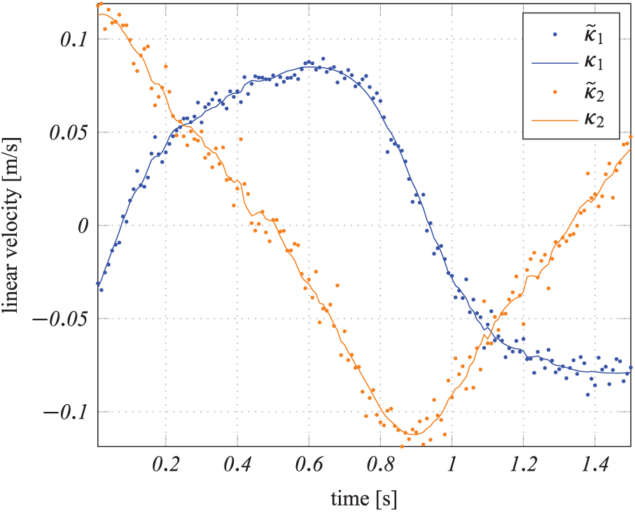
Figure 5 shows the (simulated) measured velocities in the tool’s plane $\tilde{κ} (t)$ compared with the execution of a parametrized version of $κ (w^{*}, w_{κ}^{*}, t)$ , which exploits our proposed polynomial regressors for the circular trajectories. In Figure 6, we show the equivalent result used for the joint limit avoidance for the redundant joints ( $\tilde{γ}$ versus $γ$ ). In addition to this, in Figure 7, we depict the simulated ground-truth policy (unknown to the learner, of course) and we overlay the trajectories computed using the estimated policy. In all cases, we can see that both the ground-truth values and measured values contain a noise as a consequence of a noisy wiping motion, while the reproduced estimated policies provide a filtered version of the correct values.

Fig. 5.

Planar wiping policy estimation. Estimated planar wiping policy $κ (x (t), w^{*}, w_{κ}^{*}, t)$ (continuous lines) and ground-truth planar wiping trajectory $\tilde{κ} (t)$ (dots). $\tilde{κ} (t)$ is noisy (to emulate non-perfect data from a human operator) and is not available during training.

Fig. 6.

Joint limit avoidance policy estimation. Estimated joint limit avoidance policy $γ (x (t), w^{*}, w_{γ}^{*}, t)$ (continuous lines) and ground-truth joint limit avoidance trajectory $\tilde{γ} (t)$ (dots). $\tilde{γ} (t)$ is noisy (to emulate non-perfect data from a human operator) and is not available during training.

Fig. 7.

Unconstrained policy estimation. Estimated unconstrained policy $π (x (t), w^{*}, w_{π}^{*}, (t)$ (continuous lines) and ground-truth unconstrained trajectory $\tilde{π} (t)$ (dots). $π (t)$ is noisy because $\tilde{κ} (t)$ and $\tilde{γ} (t)$ were noisy too and is not available during training. Policies corresponding to joints 2, 3, and 7 are not shown, to avoid cluttering.

7. Experimental setup

7.1. Testing with real data and a force sensor

In our experiments, we use the seven-degrees-of-freedom Kuka LWR3 robot with an ATI industrial automation Gamma force and torque sensor attached at the end effector, as shown in Figure 8. The force sensor retrieves a six-dimensional wrench vector expressed in the sensor frame. Therefore, we compute the torque at the contact point by transforming the wrench through a distance $d_{S}$ toward the contact area. We estimated this distance empirically by pressing the tool against surfaces at different angles. The robot is velocity controlled and, therefore, the minimization of the force-based main task error (equation (40)) is achieved by admittance control. This means that the robot compensates for the end-effector position and orientation according to the wrench feedback. To accommodate this motion when in contact with a rigid surface, we introduce a compliant material at the end-effector tip (such as a sponge). This added compliance introduces some dynamic behavior to the system, such as vibrations, which are suitably damped by adding a derivative component to the proportional controller suggested in the previous section.

Fig. 8.

Kuka LWR 3 robotic arm, equipped with a force and torque sensor, wiping a curved surface.

We recorded a dataset of wiping trajectories demonstrated by a human being, as shown in Figure 9. The dataset contains 12 trajectories, each on a surface at a different orientation (four of which are shown in Figure 10). Each demonstration involved several circles with the tool of the robot, giving approximately 2000 data points³ (using a sampling rate of 100 Hz). The demonstrated data were only minimally cropped to ensure that data contained only poses where the tool was in contact with the surface and moving along the demonstrated trajectory.

Fig. 9.

Demonstration of a circular wiping trajectory on a flat surface. The demonstration was repeated on 12 surfaces of different orientations.

Fig. 10.

Learning by demonstration. Four of the twelve wiping trajectories from human demonstration (green), and closed-loop policy validation using the respective flat surface orientation and initial position (blue).

We used this dataset to first learn the different constraint matrixes, by parametrizing them as a linear combination of regressors and functions of state, and by applying the estimation method described in Section 3.2. The regressors for each constraint matrix are these from equation (29). For the policy $π$ , we used 25 locally weighted models with the same regressors used by Armesto et al. (2017b). The resulting policy was then stored and used, in a closed loop, together with the force-based surface alignment task described in the previous section.

Figure 10 shows the robot’s end-effector trajectory, corresponding to the execution of the estimated null-space policy for the same constraint (surface inclination) of the demonstrations, as well as the respective end-effector position corresponding to the data. Table 1 shows the result of computing the costs J, J₁, and J₂, according to equations (11), (13), and (14), respectively. The figure shows that the locally weighted model has learned that there is a “common” circular wiping motion across the different demonstrations.

Table 1.

Costs, J, J₁, and J₂, for the four experimental demonstrations shown in Figure 10.

Demonstration	J	J ₁	J ₂
1	0.0206	0.81 × 10⁻⁶	0.0199
2	0.0445	2.36 × 10⁻⁶	0.0431
4	0.0319	2.39 × 10⁻⁶	0.0302
7	0.0199	4.43 × 10⁻⁶	0.0175

Furthermore, we have also validated the learned policy on a non-flat surface, as shown in Figure 8, demonstrating that the policy, trained from human demonstrations on flat surfaces, generalizes to both flat and curved surfaces. The resulting wiping motion is depicted in Figure 11. Note that we have demonstrated the wiping motion exclusively on flat surfaces; therefore, this shows two aspects of generalization: (I) from a surface alignment task to a force alignment task and (II) from flat surfaces to a curved surface. See Armesto et al. (2017c) for video recordings of the policy generalization to a curved surface. In many practical cases, training with flat surfaces will be easier for the demonstrator (for instance, to align the tool properly with the surface), resulting in a dataset with demonstrations in which $A (x) u \approx 0$ , and consequently reducing the amount of error in the task policy.

Fig. 11.

A wiping policy has been trained from human demonstrations on flat surfaces (without using the force sensor); the policy generalizes to non-flat surfaces using a force-sensor-based task to align the tool dynamically.

7.2. Constraint similarity analysis

In all experiments so far, we have assumed that the demonstrator provides a set of sub-datasets ${X_{1}, X_{2}, \dots, X_{ν}}$ , each of which contains samples of pairs of raw observations, which encapsulate a sufficiently diverge set of tasks and constraints, allowing us to uncover the underlying policy common to all demonstrations that, therefore, can be generalized to different constraints. To estimate the unconstrained policy, we need demonstrations from different constraints (Howard and Vijayakumar, 2007). As a consequence, a typical dataset will contain a sequence of demonstrations, which will be classified as sub-datasets.

The aim now is to analyse how similar or distinct these sub-datasets are from one another, regarding the estimated underlying constraint, by using the same cost metric proposed for the constraint estimation. Moreover, we consider this analysis for the case of a single full dataset containing data originating from different constraints, to help us in identifying the transition regions. The experiments in this section are meant to provide an additional analysis of the training data, highlighting the difference between data obtained for an unconstrained motion or a motion subject to the same constraint and data collected under different constraints.

To compare the sub-datasets, we simply compute the cost J₁ from equation (13) for the sub-dataset l using the parameters ${\hat{w}}_{k}$ estimated with the sub-dataset k, as

$J_{1, k, l} = {∥A ({\hat{w}}_{k}, t_{l}) u (t_{l}) - b ({\hat{w}}_{k}, t_{l})∥}^{2}$ (46)

where we index the time $t_{l}$ to emphasize that the data is coming from dataset l. The value of $J_{1, k, l}$ will be low for $k = l$ and high otherwise, according to the assumption that each sub-dataset was subjected to different constraints. When different constraints intersect in some region of the space, i.e., the underlying constraints are similar to one another, this cost should be low, reflecting this constraint similarity.

For the experimental data used in the previous subsection, we manually selected the ν sub-datasets. This pre-processing step separates the full dataset into the sub-datasets. Figure 12 shows the Cartesian positions of the Kuka’s end effector for the full dataset (blue) and, overlapping, the corresponding manually separated sub-datasets (red).

Fig. 12.

Kuka lightweight robotic arm end effector. Cartesian positions for a full unseparated dataset (blue), subject to different constraints in the form of flat surface inclinations. Overlapping are the manually separated sub-datasets, showing that a full unprocessed dataset contains transition regions with data points that are discarded before the learning process.

This manual separation was achieved by visually inspecting the data and selecting the initial and final indices of the data points for each sub-dataset. However, for larger full datasets this figure might become cluttered, making it difficult even to verify that some demonstrations correspond to very similar constraints. This suggests that we could use J₁ to split the sub-datasets.

Given an unprocessed dataset, we must conduct a similarity analysis for groups of data points, regardless of whether they correspond to the same constraint or not. One approach is to select a set of consecutive data points that represent a window within the full dataset. We then compute the parameters for that window k. We shift window k across the dataset by some increment smaller then the size of the window, creating a window k + 1 (the size refers to the number of consecutive data points). If the parameters estimated in this new window produce a small J₁, then this suggests that the data covered by these two windows is subjected to the same constraint.

By repeating this process for the full dataset, we then obtain a matrix such as the one shown in Figure 13. This matrix corresponds to the data shown in Figure 12. We have empirically chosen a window size of 400 samples (corresponding to 8 s for a sampling frequency of 50 Hz) and increments of 50 samples (1 s). In Figure 13, we also overlap boxes showing the manual separation provided by the expert. There are at least two groups of windows (around indices 120 and 150) that could be confused with demonstrations, given that they produce squares of small J₁ in the matrix. Even though these two groups of samples are not true demonstrations, the cost J₁ indicates that the data belonging to those two groups are consistent with some constraint, which is sufficiently well modeled by the chosen combination of regressors. For instance, if those samples correspond to a moment in time where the robot was static while changing the flat table orientation between demonstrations, then it makes sense to say that those data points are consistent with the same constraint, e.g. the same configuration of the robot. This metric can be further combined with other application specific metrics. Data points where the robot is static may be removed using pre-processing if necessary. Alternatively, a tactile sensor could be used to detect when the end tool is in contact with the surface, etc.

Fig. 13.

Normalized $J_{1, k, l}$ cost for window l using estimated parameters from window k. Each window contains 400 consecutive data points from the full unseparated dataset, differing from the preceding window by 50 data points.

8. Conclusion

This paper presents a new method for learning, from demonstration, policies that lie in the null space of a primary task, i.e. subject to some constraint. We introduce the term “constraint-aware policy learning” as a reformulation of the direct policy learning method, where the policy appropriately parametrizes the constraint. Additionally, we discuss the conditions for which this “constraint-aware policy learning” can be split into two optimization problems: constraint estimation preceded by null-space policy estimation.

The main advantage of this approach, compared with classic direct policy learning, is its ability to learn a policy consistent with the constraint. To demonstrate this point, we used different tasks and constraints in our experimental demonstration with the real Kuka lightweight arm. In this case, while recording the training data, the human demonstrator provides the task, whereas in the validation stage we use a force-based task to adapt and align the tool to an unknown surface.

While the null-space policy can be parametrized with locally weighted models, as discussed in this paper, or any other more generic functions, in the example of learning a wiping motion we choose to take advantage of our knowledge of this specific task by incorporating more specialized regressors. This decreases the number of parameters that the algorithm must learn, decreasing the required number of demonstrations. Certainly, a clever choice of regressors can—as in our case—greatly improve the results or even turn the learning exercise into a trivial problem. However, what this framework provides is a way of encapsulating all the specifics and domain knowledge in the chosen regressors, and not in the learning algorithm itself.

Moreover, we consider the case of a null-space policy that, instead of having the full dimension of the system actions, can be decomposed, by assumption, into a set of lower-dimensional policies. For this case, we propose an alternative reformulation for estimating these lower-dimensional policies, provided the respective regressors are supplied.

However, to learn a generalizable null-space policy, we must somehow guarantee that the training datasets provide enough variability of constraints. We provide a means of comparing the datasets, regarding their underlying constraint, by using the same metric used in the constraint estimation. This involves building a similarity matrix by computing the estimation residual of a sub-dataset, using the estimated parameters from the other sub-datasets. Furthermore, besides allowing us to identify similar constraints between different sub-datasets, this similarity matrix allows us to identify different constraints within the same dataset, by running the samemetric but over different windows of data. This can be a valuable tool for helping to identify the beginning and end of a demonstration.

In our future work, we intend to exploit more challenging application domains, as well as learning constrained tasks for dynamic systems. We would also like to integrate the constraint-aware learning framework with other policy learning methods to guarantee some desired properties for the null-space policy.

Footnotes

Funding

The author(s) disclosed receipt of the following financial support for the research,authorship,and/or publication of this article: This work was supported by the Spanish Ministry of Economy and the European Union (grant number DPI2016-81002-R (AEI/FEDER,UE)),the European Union Horizon 2020,as part of the project Memory of Motion - MEMMO (project ID 780684),and the Engineering and Physical Sciences Research Council,UK,as part of the Robotics and AI hub in Future AI and Robotics for Space - FAIR-SPACE (grant number EP/R026092/1),and as part of the Centre for Doctoral Training in Robotics and Autonomous Systems at Heriot-Watt University and the University of Edinburgh (grant numbers EP/L016834/1 and EP/J015040/1).

References

Alissandrakis

Nehaniv

Dautenhahn

(2007) Correspondence mapping induced state and action metrics for robotic imitation. IEEE Transactions on Systems, Man, and Cybernetics, Part B (Cybernetics) 37(2): 299–307.

Argall

Chernova

Veloso

et al . (2009) A survey of robot learning from demonstration. Robotics and Autonomous Systems 57(5): 469–483.

Armesto

Bosga

Ivan

et al . (2017a) Efficient learning of constraints and generic null space policies. In: International conference on robotics and automation, Singapore, 29 May–3 June 2017, pp. 1520–1526. Piscataway, NJ: IEEE.

Armesto

Ivan

Moura

et al . (2017b) Learning constrained generalizable policies by demonstration. In: Robotics: Science and systems (eds. Amato

Srinivasa

Nora

et al .), Cambridge, MA, USA, 12–16 July 2017. Cambridge, MA: Robotics: Science and System XIII.

Armesto

Ivan

Moura

et al . (2017c) Efficient learning of constraints and generic null space policies. Available at: https://www.youtube.com/watch?v=2n0yW1yI524 (accessed 19th June 2018).

Atkeson

Moore

Schaal

(1997) Locally weighted learning for control. Artificial Intelligence Review 11(1–5): 75–113.

Baerlocher

Boulic

(2004) An inverse kinematics architecture enforcing an arbitrary number of strict priority levels. The Visual Computer 20(6): 402–417.

Calinon

(2016) A tutorial on task-parameterized movement learning and retrieval. Intelligent Service Robotics 9(1): 1–29.

Calinon

Billard

(2007) Incremental learning of gestures by imitation in a humanoid robot. In: ACM/IEEE international conference on human–robot interaction, Arlington, VA, USA, 10–12 March 2007, pp. 255–262. New York, NY: ACM.

10.

Cruse

Brüwer

(1987) The human arm as a redundant manipulator: The control of path and joint angles. Biological Cybernetics 57(1–2): 137–144.

11.

D’Souza

Vijayakumar

Schaal

(2001) Learning inverse kinematics. In: IEEE/RSJ international conference on intelligent robots and systems, Maui, HI, USA, 29 October–3 November 2001, vol. 1., pp. 298–303. Piscataway, NJ: IEEE.

12.

Escande

Mansard

Wieber

(2014) Hierarchical quadratic programming: Fast online humanoid–robot motion generation. The International Journal of Robotics Research 33(7): 1006–1028.

13.

Gams

Nemec

Ijspeert

et al . (2014) Coupling movement primitives: Interaction with the environment and bimanual tasks. IEEE Transactions on Robotics 30(4): 816–830.

14.

Gienger

Janssen

Goerick

(2005) Task-oriented whole body motion for humanoid robots. In: IEEE-RAS international conference on humanoid robots, Tsukuba, Japan, 5 December 2005, pp. 238–244. Piscataway, NJ: IEEE.

15.

Haykin

(1998) Neural Networks: A Comprehensive Foundation (2nd edition). Upper Saddle River, NJ: Prentice Hall PTR.

16.

Herzog

Rotella

Mason

et al . (2015) Momentum control with hierarchical inverse dynamics on a torque-controlled humanoid. Autonomous Robots 40(3): 473–491.

17.

Hornik

Stinchcombe

White

(1989) Multilayer feedforward networks are universal approximators. Neural Networks 2(5): 359–366.

18.

Howard

Vijayakumar

(2007) Reconstructing null-space policies subject to dynamic task constraints in redundant manipulators. In: Workshop on robotics and mathematics (RoboMat), Coimbra, Portugal, 17–19 September 2007. Edinburgh, UK: Informatics Report Series EDI-INF-RR-1200.

19.

Howard

Klanke

Gienger

et al . (2009) A novel method for learning policies from variable constraint data. Autonomous Robots 27(2): 105–121.

20.

Hussein

Mohammed

Ali

(2015) Learning from demonstration using variational Bayesian inference. In: Ali

Kwon

Lee

al.

(eds.) Current Approaches in Applied Artificial Intelligence. IEA/AIE 2015 (Lecture Notes in Computer Science, vol. 9101). Cham: Springer, pp. 371–381.

21.

Ijspeert

Nakanishi

Schaal

(2003) Learning attractor landscapes for learning motor primitives. In: 15th international conference on neural information processing systems (eds. Becker

Thrun

Obermayer

), Vancouver, British Columbia, Canada 8–13 December 2003, pp. 1547–1554. Cambridge, MA: MIT Press.

22.

Kanungo

Mount

Netanyahu

et al . (2002) An efficient k -means clustering algorithm: Analysis and implementation. IEEE Transactions on Pattern Analysis and Machine Intelligence 24(7): 881–892.

23.

Khatib

Sentis

Park

(2008) A unified framework for whole-body humanoid robot control with multiple constraints and contacts. In: Bruyninckx

Přeučil

Kulich

(eds.) European Robotics Symposium 2008 (Springer Tracts in Advanced Robotics, vol. 44). Berlin: Springer, pp. 303–312.

24.

Lin

Howard

Vijayakumar

(2015) Learning null space projections. In: IEEE international conference on robotics and automation, Seattle, WA, USA, 26–30 May 2015, pp. 2613–2619. Piscataway, NJ: IEEE.

25.

Lin

Ray

Howard

(2017) Learning task constraints in operational space formulation. In: IEEE international conference on robotics and automation, Singapore, 29 May–3 June 2017, pp. 309–315. Piscataway, NJ: IEEE.

26.

Mansard

Chaumette

(2007) Task sequencing for high-level sensor-based control. IEEE Transactions on Robotics 23(1): 60–72.

27.

Moura

Erden

(2017) Formulation of a control and path planning approach for a cab front cleaning robot. In: Procedia CIRP 59: 67–71.

28.

Paraschos

Lioutikov

Peters

et al . (2017) Probabilistic prioritization of movement primitives. IEEE Robotics and Automation Letters 2(4): 2294–2301.

29.

Pastor

Righetti

Kalakrishnan

et al . (2011) Online movement adaptation based on previous sensor experiences. In: IEEE/RSJ international conference on intelligent robots and systems, San Francisco, CA, USA, 25–30 September 2011, pp. 365–371. Piscataway, NJ: IEEE.

30.

Schaal

Atkeson

(1998) Constructive incremental learning from only local information. Neural Computation 10(8): 2047–2084.

31.

Schaal

Ijspeert

Billard

(2003) Computational approaches to motor learning by imitation. Philosophical Transactions of the Royal Society B: Biological Sciences 358(1431): 537–547.

32.

Shiller

(2015) Off-line and on-line trajectory planning. In: Carbone

Gomez-Bravo

(eds.), Motion and Operation Planning of Robotic Systems: Background and Practical Approaches (Mechanisms and Machine Science, vol. 29). Cham: Springer International Publishing, pp. 29–62.

33.

Siciliano

Sciavicco

Villani

et al . (2009) Differential Kinematics and Statics. London: Springer, pp. 105–160.

34.

Sugiura

Gienger

Janssen

et al . (2006) Real-time self collision avoidance for humanoids by means of nullspace criteria and task intervals. In: IEEE-RAS international conference on humanoid robots, Genova, Italy, 4–6 December 2006, pp. 575–580. Piscataway, NJ: IEEE.

35.

Towell

Howard

Vijayakumar

(2010) Learning nullspace policies. In: IEEE/RSJ international conference on intelligent robots and systems (IROS), Taipei, Taiwan, 18–22 October 2010, pp. 241–248. Piscataway, NJ: IEEE.

36.

Yoshikawa

(1985) Manipulability of robotic mechanisms. The International Journal of Robotics Research 4(2): 3–9.

37.

Zhang

(2017) Matrix Analysis and Applications. Cambridge: Cambridge University Press.