Adaptively Informed Trees (AIT*) and Effort Informed Trees (EIT*): Asymmetric bidirectional sampling-based path planning

Abstract

Optimal path planning is the problem of finding a valid sequence of states between a start and goal that optimizes an objective. Informed path planning algorithms order their search with problem-specific knowledge expressed as heuristics and can be orders of magnitude more efficient than uninformed algorithms. Heuristics are most effective when they are both accurate and computationally inexpensive to evaluate, but these are often conflicting characteristics. This makes the selection of appropriate heuristics difficult for many problems. This paper presents two almost-surely asymptotically optimal sampling-based path planning algorithms to address this challenge, Adaptively Informed Trees (AIT*) and Effort Informed Trees (EIT*). These algorithms use an asymmetric bidirectional search in which both searches continuously inform each other. This allows AIT* and EIT* to improve planning performance by simultaneously calculating and exploiting increasingly accurate, problem-specific heuristics. The benefits of AIT* and EIT* relative to other sampling-based algorithms are demonstrated on 12 problems in abstract, robotic, and biomedical domains optimizing path length and obstacle clearance. The experiments show that AIT* and EIT* outperform other algorithms on problems optimizing obstacle clearance, where a priori cost heuristics are often ineffective, and still perform well on problems minimizing path length, where such heuristics are often effective.

1. Introduction

Path planning algorithms aim to find a sequence of valid states, called a path, that connects a start to a goal. Sampling-based planners, such as Probabilistic Roadmaps (PRM; Kavraki et al., 1996), find paths by randomly sampling valid states and connecting nearby states when these local connections are valid. The resulting structure can be viewed as a graph embedded in a state space, where each vertex represents a valid state and each edge a sequence of valid states connecting two vertices. Multiple planning problems can be solved by adding starts and goals to this embedded graph and then finding a path between them with a graph-search algorithm.

A single planning problem is often solved more efficiently with incremental sampling-based planners, such as Rapidly-exploring Random Trees (RRT; LaValle and Kuffner Jr 1999, 2001) and its asymptotically optimal variant, RRT* (Karaman and Frazzoli 2010, 2011). These planners build a search tree of valid paths rooted at the start by incrementally sampling and connecting states when these local connections are valid. This avoids having to specify the sampling resolution a priori, but results in a randomly ordered search that spends computational effort on paths that are never part of a solution.

Best-first graph-search algorithms, such as Dijkstra’s algorithm (Dijkstra 1959), can search problems more efficiently by ordering their search on partial solution cost. Informed graph-search algorithms, such as A* (Hart et al., 1968), can further increase search efficiency by leveraging problem-specific information to order their search on total potential solution cost. This information is often expressed as a heuristic function that estimates the cost to connect any two vertices in a graph. A heuristic is called admissible if it never overestimates the true cost and consistent if it satisfies a specific triangle inequality. Given an admissible cost heuristic, A* finds an optimal solution, and given a consistent cost heuristic, A* does so optimally efficiently with respect to the number of expanded vertices (Dechter and Perl, 1985).

The efficient search order of A* is combined with the incremental sampling of RRT* in informed sampling-based planners, such as Batch Informed Trees (BIT*; Gammell et al., 2015, 2020). This improves planning performance, but only when effective cost heuristics are available. A heuristic is most effective when it is both accurate and computationally inexpensive to evaluate relative to other search operations. Such heuristics may not exist for some problems, because they are inaccurate for a given obstacle configuration or computationally expensive due to complex optimization objectives, or may not be admissible, which is often required for theoretical performance guarantees of informed planners.

Problem-specific information not expressible as admissible cost heuristics can be exploited by more advanced informed graph-search algorithms, such as Anytime Explicit Estimation Search (AEES; Thayer et al., 2012) and Anytime Multi-Heuristic A* (A-MHA*; Natarajan et al., 2019). These algorithms decouple search order from solution quality guarantees, which allows them to balance search efficiency with anytime performance. This is especially important for robotic systems that operate under hard time constraints.

This paper presents techniques to inexpensively calculate accurate, admissible, and problem-specific heuristics and exploit them with sampling-based planning algorithms. This is achieved with an asymmetric bidirectional search that considers different information in the forward and reverse searches. These two searches continuously inform each other by sharing complementary information in both directions. Algorithm 1 provides a conceptual overview of this approach.

The reverse search calculates heuristics for the current sampling-based approximation of a planning problem. It exploits problem-specific information implicit in the observed distribution of valid states by combining a priori heuristics between multiple states into more accurate heuristics between each state and the goal. The reverse search is computationally inexpensive because it only combines edge heuristics and avoids full collision detection and true edge cost evaluation.

The forward search finds valid paths in the current sampling-based approximation of a planning problem. It does this effectively by exploiting the accurate, problem-specific heuristics calculated by the reverse search. The forward search informs the reverse search when invalid edges were used to calculate the heuristic, causing the reverse search to update the heuristic. The forward search is computationally expensive because it performs full collision detection and edge cost evaluation, but focused on connections likely to yield a solution by the calculated heuristics (Figure 1).

Figure 1.

An illustration of the search trees constructed by RRT*, FMT*, BIT*, AIT*, and EIT* to find an initial solution when optimizing path length (a–e) and obstacle clearance (f–j). The start and goal are represented by a black dot and circle, respectively. Sampled states are represented by small black dots. State space obstacles are indicated with gray rectangles. The initial solutions are shown in yellow and the search trees constructed to find them are shown in black. Any edge in these search trees that is not part of the initial solution delayed finding it. RRT* randomly explores the state space and fully evaluates many edges that are not part of the initial solution for both objectives (a, f). FMT* orders its search with increasing cost-to-come of the vertices and not only fully evaluates many edges that are not part of the initial solution for both objectives but also fails to find a solution when optimizing obstacle clearance because its connection strategy depends on edge cost (b, g). BIT* orders its search on the total potential solution cost according to an admissible cost heuristic and evaluates fewer edges that are not part of the initial solution (c) but only if an informative admissible cost heuristic is available (h). AIT* calculates and exploits a problem-specific heuristic and evaluates still fewer edges that are not part of the initial solution (d) but only when an informative admissible cost heuristic can be calculated for the optimization objective (i). EIT* calculates and exploits cost and effort heuristics and evaluates few edges even when an admissible cost heuristic cannot be calculated for the objective (e, j).

This paper presents two almost-surely asymptotically optimal sampling-based planning algorithms informed by an asymmetric bidirectional search, Adaptively Informed Trees (AIT*) and Effort Informed Trees (EIT*). AIT* calculates an increasingly accurate, admissible cost heuristic with its reverse search and exploits this heuristic with its forward search. This results in fast initial solution times even when the admissible cost heuristic available a priori is not accurate. The full details of AIT* are presented in Section 3.2.

EIT* builds on AIT* by calculating an additional cost and effort heuristic with its reverse search and exploiting all three heuristics with its forward search. This results in fast initial solution times even when no admissible cost heuristic is available. The full details of EIT* are presented in Section 3.3.

The benefits of simultaneously calculating and exploiting adaptive heuristics are demonstrated on 12 problems in abstract, robotic, and biomedical domains in Section 4. All domains are tested with the path-length objective, where informative admissible heuristics are available a priori, and the obstacle-clearance objective, where informative admissible heuristics are not always available a priori. The results show that EIT* outperforms all other asymptotically optimal planners on all problems in all domains when optimizing obstacle clearance. AIT* and EIT* also perform well when minimizing path length in comparison to the tested planners when considering success rates, median initial solution times, and median solution quality over time.

1.1. Statement of Contributions

This paper expands on ideas first published as Strub and Gammell (2020a). It makes the following specific contributions:

• Presents EIT* as an extension of AIT* to optimization objectives that are computationally expensive or difficult to approximate with an admissible a priori cost heuristic (Section 3.3).

• Proves the almost-sure asymptotic optimality of these algorithms by building on results from the path-planning and graph-search literature (Section 3.3).

• Demonstrates the effectiveness of these algorithms across multiple domains and optimization objectives, including problems of robotic manipulation and problems with continuous goal regions (Section 4).

2. Background

This section first formally defines the optimal path planning problem (Section 2.1) and then reviews related techniques from the literature on using heuristics in sampling-based planners and graph-search algorithms (Section 2.2).

2.1. Problem Definition

There are two widely studied versions of the path planning problem. The feasible path planning problem is the task of finding a sequence of valid states, i.e., a path, that leads from a start to a goal. Many feasible problems have many solutions. The optimal path planning problem is the task of finding the best among these solutions, i.e., a valid path that is optimal with respect to a given optimization objective. Many optimal problems have a unique solution. The optimal path planning problem is formally defined in Definition 1.

Definition 1

The Optimal Path Planning Problem (Karaman and Frazzoli 2011). Let the state space of a planning problem be denoted by X, the subset of invalid states by X_invalid ⊂ X, and the subset of valid states by $X_{\text{valid}}:=\text{closure}\left(X/X_{\text{invalid}}\right)$ . Let the start state and the set of goal states be denoted by x_start ∈ X_valid and X_goal ⊂ X_valid, respectively. Let σ: [0, 1] → X_valid be a continuous function with bounded total variation, i.e., a valid path, and let the set of all valid paths be denoted by Σ. Let the optimization objective be defined by a cost function, c: Σ → [0, ∞), that maps each path to a nonnegative real number.

The optimal path planning problem is the task of finding a path, σ* ∈ Σ, from the start to the goal with minimum cost, $${\sigma }^{\ast }:=\underset{\sigma \in \mathrm{\Sigma }}{\text{argmin}}\left\{c\left(\sigma \right)|\sigma \left(0\right)={\mathbf{x}}_{\text{start}},\sigma \left(1\right)\in X_{\text{goal}}\right\},$$ or reporting failure if no such path exists.

Algorithm 1

Asymmetric bidirectional search

1 repeat

2 improve RGG approximation (sampling)

3 calculate heuristics (reverse search)

4 while RGG approximation is useful do

5  find solution (forward search)

6  if found invalid edge or unprocessed state

7   update heuristics (reverse search)

8 until stopped

Sampling-based planners are often evaluated probabilistically as a function of the number of samples over all possible realizations of a distribution. Algorithms whose probability of solving the feasible path planning problem approaches one as the number of samples approaches infinity are called probabilistically complete. Algorithms that asymptotically solve the optimal planning problem as the number of samples approaches infinity with a probability of one are called almost-surely asymptotically optimal (Karaman and Frazzoli 2011). Almost-sure asymptotic optimality implies probabilistic completeness and is formally defined in Definition 2.

Definition 2

Almost-sure asymptotic optimality (Karaman and Frazzoli 2011). A sampling-based path planning algorithm is called almost-surely asymptotically optimal if it has a unity probability of asymptotically solving the optimal path planning problem as the number of samples approaches infinity (if an optimal solution exists), $$P\left(\underset{q\to \infty }{\text{lim}\hspace{0.17em}\text{sup}}\underset{\sigma \in {\mathrm{\Sigma }}_q}{\min }\left\{c\left(\sigma \right)\right\}=c^{\ast }\right)=1,$$ where q is the number of samples, Σ _q ⊂ Σ is the set of valid paths from the start to the goal found by the planner from those samples, c: Σ → [0, ∞) is the cost function, and c* is the optimal solution cost.

Sampling-based planners can also use deterministic sampling strategies (e.g., Branicky et al., 2001; LaValle et al., 2004), which can result in deterministic optimality guarantees (Janson et al., 2018). The finite-time properties of asymptotically optimal planners are analyzed by Dobson and Bekris (2013), Janson et al. (2018), and Tsao et al. (2020).

Formally analyzing sampling-based planners requires assumptions about the path planning problem (e.g., Gammell and Strub 2021). The analysis of AIT* and EIT* builds on the probabilistic results of Karaman and Frazzoli (2011) and makes the same assumptions (Sections 2.1.1–2.1.4).

2.1.1. State space assumption

The state space of the planning problem is assumed to be an open, n-dimensional unit (hyper)cube, X := (0, 1)ⁿ, but problems with other state spaces can also be searched (Kleinbort et al., 2016; 2020b).

2.1.2. Cost function assumptions

Let σ₁, σ₂ ∈ Σ be two paths such that σ₁(1) = σ₂(0), and let (σ₁|σ₂) ∈ Σ denote their concatenation, $$\left({\sigma }_1|{\sigma }_2\right)\left(t\right):=\{\begin{array}{ll}{\sigma }_1\left(2t\right)\hfill & \text{for }t\in \left[0,\frac{1}{2}\right]\hfill \\ {\sigma }_2\left(2t-1\right)\hfill & \text{for }t\in \left[\frac{1}{2},1\right].\hfill \end{array}$$

The cost of any path, σ = (σ₁|σ₂) ∈ Σ, is assumed to be lower bounded by the cost of any of its segments, $$\forall {\sigma }_1,{\sigma }_2\text{ s}\text{.t}\text{. }\sigma =\left({\sigma }_1|{\sigma }_2\right),\hspace{1em}c\left(\sigma \right)\ge \max \left\{c\left({\sigma }_1\right),c\left({\sigma }_2\right)\right\},$$ and upper bounded by a multiple of its total variation, $$\exists k\in \left(0,\infty \right),\hspace{1em}c\left(\sigma \right)\le k\text{TV}\left(\sigma \right),$$ where TV(σ) denotes the total variation of the path σ (Karaman and Frazzoli 2011).

It is also assumed that only trivial paths consisting of a single state can have zero cost, $$c\left(\sigma \right)=0\iff \forall t\in \left[\mathrm{0,1}\right],\sigma \left(t\right)=\sigma \left(0\right).$$

2.1.3. Obstacle Assumption

The obstacle configuration of the optimal path planning problem is assumed to allow for a valid path from the start to the goal that remains a fixed distance, δ > 0, from its nearest obstacles for its entire length, $$\exists \sigma \in \mathrm{\Sigma },\delta \in \left(0,\infty \right),\text{s}\text{.t}\text{. }\forall t\in \left[\mathrm{0,1}\right],B_{\delta ,n}\left(\sigma \left(t\right)\right)\subset X_{\text{valid}},$$ where B _{δ ,n} (σ(t)) is an n-dimensional ball with radius δ centered at σ(t), $$B_{\delta ,n}\left(\mathbf{x}\right):=\left\{{\mathbf{x}}^{\prime }\in X|\mathrm{\Vert }\mathbf{x}-{\mathbf{x}}^{\prime }{\mathrm{\Vert }}_2\le \delta \right\}.$$ Such a path is said to have strong δ-clearance.

2.1.4. Optimal Solution Assumption

At least one solution of the optimal path planning problem, σ* ∈ Σ, is assumed to be homotopic to a path, σ _δ ∈ Σ, with strong δ-clearance, $$\exists H:\left[\mathrm{0,1}\right]\to \mathrm{\Sigma },\hspace{1em}H\left(0\right)={\sigma }^{\ast },H\left(1\right)={\sigma }_{\delta },$$ where H is a homotopic map whose image is the set of all valid paths from the start to the goal. Such a solution is said to have weak δ-clearance.

2.2. Literature Review

Almost-surely asymptotically optimal planning is a popular area of research (Gammell and Strub 2021). This section focuses on sampling-based and graph-search techniques to calculate and/or exploit heuristics to improve performance. Sampling-based planners that use heuristics to guide the sampling and/or order the search are reviewed in Section 2.2.1. Approaches that calculate and exploit accurate cost heuristics for graph-search algorithms are reviewed in Section 2.2.2 and algorithms that use effort heuristics in Section 2.2.3. Using heuristics in sampling-based planning has parallels with lazy collision detection, which is reviewed in Section 2.2.4.

2.2.1. Heuristics in Sampling-Based Planning

Sampling-based planning algorithms can improve their performance by using heuristics to bias their sampling and guide their search.

RRT-Connect (Kuffner Jr and LaValle 2000) builds on RRT by growing two trees, one rooted in the start and one in the goal state. These trees each explore the state space around them, but are also guided towards each other with a connect heuristic. This approach can result in very fast initial solution times, but does not consider the solution cost and can consequently not improve the solution given more computational time. Almost-surely asymptotically optimal variants of RRT-Connect exist (Akgun and Stilman 2011; Burget et al., 2016; Jordan and Perez 2013; Klemm et al., 2015; Qureshi and Ayaz 2015), but the connect heuristic does not guide the search beyond finding an initial solution.

Heuristically-Guided RRT (hRRT; Urmson and Simmons 2003) and Generalized Bidirectional RRT (GBRRT; Nayak and Otte 2021) bias the growth of their trees with cost heuristics. hRRT uses a priori heuristics to weigh the Voronoi regions of RRT. GBRRT is a bidirectional version of RRT that guides the forward tree with heuristics computed by the reverse tree. These algorithms have improved performance but do not provide any bounds on the quality of their solution.

Informed RRT* (Gammell et al., 2014, 2018) builds on RRT* by using an admissible cost heuristic to ensure that only states that can improve the current solution are processed. This improves RRT*’s convergence rate and retains its almost-sure asymptotic optimality, but does not guide the search with the heuristic, does not improve the accuracy of the heuristic as the search progresses, and does not provide any benefits until an initial solution is found. Kunz et al. (2016) and Yi et al. (2018) extend informed sampling to kinodynamic systems. Joshi and Tsiotras (2019) present a variant of Informed RRT* that uses previous collision detection results and available information in the graph structure to guide the search.

RRT^# (Arslan and Tsiotras 2013, 2015) builds on RRT* by ensuring that all samples are optimally connected to the search tree after each iteration. It does this efficiently by using an admissible cost heuristic to update the connections of suboptimally connected samples in order of their total potential solution cost. This again improves RRT*’s convergence rate and retains its almost-sure asymptotic optimality, but can also not improve the accuracy of the heuristic as the search progresses and does not provide any benefits until an initial solution is found.

Sakcak et al. (2020) present a method that incorporates a heuristic into a version of RRT* that is based on motion primitives (Sakcak et al., 2019). This can improve the performance on kinodynamic problems but uses a discretization of the state space that suffers from the curse of dimensionality (Bellman 1957).

Informed Subdivision Tree (IST; Bekris and Kavraki 2008), A*-RRT (Li and Bekris 2011), the f-biasing method (Kiesel et al., 2012), P-PRM (Le and Plaku 2014), and Region Informed Optimal Trees (RIOT; Westbrook and Ruml 2020) all search a simplified approximation of the state space to calculate an accurate cost heuristic, which is then used to guide a sampling-based planner. These approaches improve planning performance but require a preprocessing step.

Bayesian Effort-Aided Search Trees (BEAST; Kiesel et al., 2017) is similar to these methods in that it runs PRM on a simplified abstraction of the problem and uses the resulting graph to calculate an effort heuristic for the samples in the simplified space. If searching the original space reveals that regions in the abstract space cannot easily be connected, then this effort heuristic is updated in a Bayesian manner. BEAST tends to find initial solutions faster than other planners but does not provide any guarantees on the quality of its solutions.

Quotient-space RoadMap Planner (QMP; Orthey et al., 2018), Quotient-space RRT (QRRT; Orthey and Toussaint 2019), and their asymptotically optimal variants QMP* and QRRT* (Orthey and Toussaint 2019) solve planning problems with sequences of admissible lower-dimensional simplifications of increasing dimensionality. Paths in lower-dimensional simplifications can guide the sampling of states in higher dimensional simplifications and can be seen as admissible heuristics. This can improve performance by orders of magnitude, especially for high-dimensional problems, but requires the user to manually specify the sequence of lower-dimensional simplifications for each problem.

Motion Planning using Lower Bounds (MPLB; Salzman and Halperin 2015) is an anytime adaption of Fast Marching Trees (FMT*) (Janson and Pavone 2013; Janson et al., 2015) that incorporates admissible cost heuristics. MPLB uses two passes of Dijkstra’s algorithm to restrict the set of samples to be searched and another pass of Dijkstra’s to calculate an admissible cost heuristic for these samples, all without detecting collisions. It then uses the resulting cost heuristic in a forward search with collision detection to find a path. This approach can result in accurate, admissible cost heuristics and requires few collision detections but does not update the heuristic when the forward search detects collisions on edges that were used to compute the heuristic.

BIT* samples batches of states and views these states as an increasingly dense edge-implicit Random Geometric Graph (RGG; Penrose 2003). It uses an admissible cost heuristic to search this graph in order of potential solution quality with techniques similar to Lifelong Planning A* (LPA*; Koenig et al., 2004; Likhachev and Koenig 2005; Aine and Likhachev 2016). Advanced BIT* (ABIT*; Strub and Gammell 2020b) speeds up initial solution times by inflating its heuristic, similar to Anytime Repairing A* (ARA*; Likhachev et al., 2004), and balances exploring the state space with exploiting the current RGG approximation by truncating its search, similar to Truncated LPA* (TLPA*; Aine and Likhachev 2016). Both algorithms work best when the cost of a path correlates well with the computational effort required to validate it and when accurate cost heuristics are available a priori, but require that these heuristics are admissible and do not improve their accuracy as the search progresses.

Similar to AIT* and EIT*, the methods in this section use heuristics to improve the performance of sampling-based planning algorithms. In contrast to AIT* and EIT*, these methods either do not apply heuristics to all aspects of the search, do not provide any bounds on the quality of their solution, require a preprocessing step, do not calculate problem-specific heuristics, or do not improve the accuracy of the heuristic as the search progresses.

2.2.2. Improved heuristics in graph-search

Developing and exploiting accurate heuristics is an important area of research in informed graph-search algorithms. Techniques to calculate more accurate heuristics have improved performance in various problem domains, e.g., the 15-Puzzle (Culberson and Schaeffer 1996), Rubik’s Cube (Korf 1997), and robot vacuum on a grid (Thayer et al., 2011).

Pattern databases (Culberson and Schaeffer 1996, 1998; Korf 1997) are precomputed tables of exact solution costs to potentially simplified subproblems of a problem domain. The highest solution cost of any remaining subproblem in an ongoing search can be used as an accurate heuristic for an informed search. Additive pattern databases (Felner et al., 2004) are constructed such that the heuristic remains admissible when the solution costs of all remaining subproblems are combined, which can result in more accurate heuristics. This increased accuracy can significantly improve performance, but is confined to problem domains for which pattern databases can be generated.

Hierarchical A* (HA*; Holte et al., 1996) uses homomorphic transformations of the state space to create abstractions in which multiple states of the original space are mapped to a single state in abstract space. These abstractions are then searched to calculate a heuristic for the original state space. This can result in fewer expanded states, but the presented technique is only shown to work for graphs with uniform edge costs. Hierarchical Cooperative A* (HCA*; Silver 2005) and Windowed HCA* (WHCA*; Silver 2005) are multiagent versions of HA* that use Reverse Resumable A* (RRA*; Silver 2005) to search the abstraction from the goal to the start. The cost of the optimal paths to states from the goal in the abstract space is used as the heuristic for the corresponding states in the original space. If the search in the original space processes a state whose abstract representation has not been processed by RRA*, then RRA* is resumed until it finds the optimal path to an abstract state that corresponds to the state being processed by the search in the original space. This results in lower cost paths and better success rates than alternative multi-agent search algorithms, but cannot directly be applied to single-agent planning in continuous spaces.

Adaptive A* (AA*; Koenig and Likhachev 2005; Sun et al., 2008) is an incremental search algorithm that calculates an increasingly accurate, admissible cost heuristic for subsequent searches of a graph with the same goal but different start states. After each search, the heuristic cost-to-go value of each closed state is updated to be the difference between the solution cost and the cost-to-come value of that state. This results in increasingly efficient searches of any problem domain but does not provide any benefits for the initial search of a graph.

The method in Thayer et al. (2011) also generates more accurate heuristics for any domain. It uses a relationship between the cost-to-go of a state and the cost-to-go of its best child to define a single-step error in the cost heuristic. The mean single-step error in this heuristic is then calculated either globally or per branch and used to adjust the heuristic accordingly. This approach can be used in the initial search but is not guaranteed to produce admissible heuristics.

The Add method (Kaindl and Kainz 1997) uses a bidirectional search in which a partial reverse search generates heuristics that inform the forward search. The reverse search reveals errors in the heuristic values of the processed states, the minimum of which is added to the heuristic values of all unexpanded states in the forward search. This results in a more informed heuristic that remains admissible, but increases the heuristic value for all unexpanded states uniformly and requires a user-defined parameter that specifies how many states to expand in the reverse search. A version without this parameter is presented by Wilt and Ruml (2013).

Similar to AIT* and EIT*, the methods in this section generate increasingly accurate heuristics that result in increasingly efficient searches. In contrast to AIT* and EIT*, these methods either require preprocessing, cannot be used for the initial search of a graph, result in inadmissible heuristics, or increase the heuristic value for all unexpanded states uniformly and only order by estimated solution cost.

2.2.3. Effort heuristics in graph-search

Ordering the search based on (inflated) cost heuristics improves anytime performance the most when the cost of a path correlates well with the computational effort required to find it (Wilt and Ruml 2012). Directly ordering the search on the computational effort of a path can instead improve performance even when this is not the case. The graph-search literature often uses the number of states that must be expanded to find a solution as a proxy for the total search effort.

Dynamically Weighted A* (DWA*; Pohl 1973) aims to improve performance by ordering its search in a manner that rewards progress away from the start. It multiplies an admissible cost heuristic by a weighting factor that decreases with increasing depth in the search tree. This is shown to reduce the number of expanded states on some problem domains, but requires an a priori estimate of the solution depth and implicitly assumes that every step away from the start is a step closer to the goal. Revised DWA* (Thayer and Ruml 2009) removes this assumption, but still requires an a priori estimate of the solution depth.

${\text{A}}_{\epsilon }^{\ast }$ (Pearl and Kim 1982) aims to expand states that are as close to the goal as possible and could be part of a solution whose cost is within a user-specified factor of the optimal cost. It always expands the node with the least number of states left to be expanded, provided it could be part of a solution within the suboptimality bound according to an admissible cost heuristic. This works well if loose suboptimality bounds are acceptable or a very accurate cost heuristic is available, but otherwise forces the search to expand states with a large estimate of states left to be expanded just to increase the lower bound on the optimal solution cost.

Explicit Estimation Search (EES; Thayer and Ruml 2011) aims to always expand the node which most quickly leads to a solution whose cost is within a user-specified bound of the optimal cost. It uses an admissible cost heuristic to guarantee the bound on the suboptimality and inadmissible cost and effort heuristics to guide its search. This significantly improves search performance in domains where solution cost and depth can differ, but introduces computational overhead and algorithmic complexity because EES must maintain three queues ordered on three different quantities. AEES is an anytime version of EES and provides the foundation of the forward search of EIT*, which is discussed in Section 3.3.2.

Similar to AIT* and EIT*, the methods in this section use estimates of the computational effort required to discover a solution to guide the search and improve performance. In contrast to AIT* and EIT*, these methods do not increase the accuracy of their heuristics as the search progresses.

2.2.4. Lazy collision detection

A byproduct of using heuristics in sampling-based planning to bias the sampling and guide the search is often that fewer edges have to be fully evaluated (Figure 1). This relates informed path planning algorithms to algorithms with lazy collision detection that explicitly aim to minimize the number of collision detections.

Lazy PRM (Bohlin and Kavraki 2000) and Fuzzy PRM (Nielsen and Kavraki 2000) take similar approaches to minimizing computational effort through lazy collision detection. Both algorithms initially connect samples without performing any collision detection on the edges. The resulting graph is processed with an informed graph-search algorithm to find a path that connects the start and goal states, and only checked for collision once a path is found. If collisions are detected, then the corresponding vertices and edges are removed from the graph and the updated graph is processed again to find a new path between the start and goal states. This results in few fully evaluated edges and improved planning performance, but Lazy PRM and Fuzzy PRM do not provide any guarantee on the quality of its solution and do not improve the accuracy of the heuristic used in their graph-search algorithm. Almost-surely asymptotically optimal variants of similar approaches exist (Hauser 2015; Kim et al., 2018) but these algorithms also do not improve the accuracy of their heuristics as the search progresses.

The Single-Query, Bi-Directional, Lazy Collision Detection (SBL) planner (Sánchez and Latombe 2003) combines lazy collision detection with ideas from RRT-Connect. It grows two trees, similar to RRT-Connect, but only checks collisions on edges that it believes to be on a path connecting the start and goal states, like Lazy PRM and Fuzzy PRM. SBL achieves fast solution times, but does also not provide any guarantees on the quality of its solution and does not improve its solution given more computational time.

Lower Bound Tree-RRT (LBT-RRT; Salzman and Halperin 2014, 2016) extends RRT* with a graph whose edges are not fully evaluated and uses this graph to determine which edges to evaluate next. LBT-RRT is almost-surely asymptotically near-optimal and allows for continuous interpolation between RRT and Rapidly-exploring Random Graphs (RRG; Karaman and Frazzoli 2011) by only rewiring states that are ɛ-inconsistent. A similar approach is used for replanning in dynamic environments in RRT^X (Otte and Frazzoli 2015, 2016). Interpolating LBT-RRT between RRT and RRG allows for balancing exploration with exploitation, but LBT-RRT can only optimize path length.

The Lazy Shortest Path (LazySP) Framework (Dellin and Srinivasa 2016) explicitly aims to minimize the number of edges that are checked for collision. It first finds a path from the start to the goal using a heuristic for the edge cost and then uses an edge selector to determine the order in which the edges on the potential solution path are checked for collision. This often results in few fully evaluated edges, but is not asymptotically optimal and restarts the search every time an edge is found to be invalid. Generalized Lazy Search (GLS; Mandalika et al., 2019) builds on LazySP by presenting a framework that can algorithmically balance edge evaluation with continuing the search, but is also not asymptotically optimal. Lazy Receding Horizon A* (LRHA*; Mandalika et al., 2018) is an example algorithm that fits within the LazySP and GLS frameworks.

Similar to AIT* and EIT*, the methods in this section improve performance by reducing the number of full edge evaluations. In contrast to AIT* and EIT*, these methods either do not use heuristics, do not improve the accuracy of their heuristics, do not guarantee any bounds on the quality of their solution, do not improve their solution given more computation time, or can only optimize path length.

3. AIT* and EIT*

AIT* and EIT* are almost-surely asymptotically optimal path planning algorithms that build on BIT*. BIT* approximates the state space with a batch of samples, which it views as an edge-implicit RGG. BIT* searches this RGG in order of the total potential solution quality of its edges until it can guarantee that it has found the resolution-optimal solution, i.e., the optimal solution in the current approximation of the state space (for other notions of resolution-optimality see, e.g., Fu et al. 2021). Once the search is finished, BIT* improves its RGG approximation by adding a new batch of samples. In this way, BIT* approximates and searches a continuously valued state space by building and searching a series of increasingly dense, edge-implicit RGGs.

To find solutions, BIT* processes the implicit edges of its current RGG approximation in order of their total potential solution cost, using incremental search techniques similar to an edge-queue version of TLPA*. It estimates the total potential solution cost of an edge as the sum of the current cost to come to the source of the edge, a heuristic estimate of the edge cost, and a heuristic estimate of the cost to go from the target of the edge. The formal guarantees of BIT* require that these cost heuristics are admissible.

AIT* and EIT* extend BIT* with an asymmetric bidirectional search that unifies many of the benefits reviewed in Section 2.2 by leveraging information implicit in the observed distribution of valid states (Figure 2). The reverse searches of AIT* and EIT* calculate accurate heuristics which are exploited by their forward searches. The forward searches in turn inform the reverse searches if they used invalid edges to compute the heuristic. In this way, both searches continuously inform each other with complementary information.

Figure 2.

An illustration of how AIT* and EIT* leverage the observed distribution of valid states to calculate accurate, problem-specific heuristics. The start and goal are represented by a black dot and circle, respectively. Sampled states are represented by small black dots. The state space obstacle is indicated with a gray rectangle. Euclidean distance is often used as a cost heuristic when optimizing path length (a, b). It suggests the green and red edges are equally promising, even though the red edge leads to a dead end (a). Calculating a problem-specific cost heuristic with a reverse search reveals that the green edge is more promising and can lead the forward search around the obstacle without evaluating many unnecessary edges (b). Some optimization objectives may not easily allow for informative admissible heuristics, such as obstacle clearance (c, d). Most informed search algorithms are ordered by cost-to-come in the absence of an informative heuristic, which again suggests that the green and red edges are equally promising (c). Calculating a problem-specific effort heuristic with a reverse search again reveals that the green edge can lead to a solution faster than the red edge, even in the absence of an informative admissible cost heuristic (d).

The reverse searches of AIT* and EIT* evaluate edges approximately and are therefore computationally inexpensive. The forward searches of AIT* and EIT* evaluate edges fully and are therefore computationally expensive, but focused by the calculated problem-specific heuristics. This computational asymmetry avoids the inefficiency of naive symmetric bidirectional informed search, where frontiers of expensive searches pass each other (Section 10.2, Pohl 1969).

An overview of the search algorithms used in AIT* and EIT* is provided in Table 1. The rest of this section presents the notation used in this paper (Section 3.1), the algorithmic details of AIT* and EIT* (Sections 3.2 and 3.3), and the formal analysis of their asymptotic optimality (Section 3.4).

Table 1

An overview of the components in BIT*, AIT*, and EIT*. All three algorithms approximate the state space with the same series of increasingly dense RGGs. BIT* does not have a reverse search and finds valid paths with an edge-queue version of TLPA* ordered by the total potential solution cost according to an a priori admissible cost heuristic. AIT* calculates a problem-specific admissible cost heuristic with a reverse LPA* search ordered by the total potential solution cost according to an a priori admissible cost heuristic. It finds valid paths with an edge-queue version of A* ordered by the total potential solution cost according to the cost heuristic calculated by its reverse search. EIT* calculates problem-specific admissible and inadmissible cost and effort heuristics with a reverse A* search ordered by the total potential solution cost and effort according to a priori cost and effort heuristics. It finds valid paths with an edge-queue version of AEES ordered by the total potential solution cost and effort according to the heuristics calculated by its reverse search. The reverse and forward search algorithms of AIT* and EIT* are detailed in Sections 3.2 and 3.3, respectively.

Component		BIT*	AIT*	EIT*
Approximation		Series of RGGs	Series of RGGs	Series of RGGs
Reverse search	Purpose	—	Calculate admissible cost heuristic	Calculate in-/admissible cost and effort heuristics
	Algorithm	—	Vertex-queue LPA*	Edge-queue A*
	Ordering	—	A priori admissible solution cost	A priori admissible solution cost and effort
	Validation	—	None	Adaptive sparse collision detection
Forward search	Purpose	Find valid paths	Find valid paths	Find valid paths
	Algorithm	Edge-queue TLPA*	Edge-queue A*	Edge-queue AEES
	Ordering	a priori admissible solution cost	Calculated admissible solution cost	Calculated in-/admissible solution cost and effort
	Validation	Dense collision detection	Dense collision detection	Dense collision detection

3.1. Notation

The state space is denoted by $X\subseteq {ℝ}^n,n\in \mathbb{N}$ , the invalid states by X_invalid ⊂ X, and the valid states by $X_{\text{valid}}:=\text{closure}\left(X/X_{\text{invalid}}\right)$ . A single state is denoted by x ∈ X. The start and goal are denoted by x_start ∈ X_valid and X_goal ⊂ X_valid, respectively. The set of sampled states underlying the RGG approximation is denoted by X_sampled ⊂ X_valid.

The forward and reverse search trees are denoted by $\mathrm{ℱ}=(V_{\mathrm{ℱ}},E_{\mathrm{ℱ}})$ and $\mathrm{ℛ}=(V_{\mathrm{ℛ}},E_{\mathrm{ℛ}})$ , respectively. All vertices in these trees, $V_{\mathrm{ℱ}}$ and $V_{\mathrm{ℛ}}$ , are individually associated with a sampled state and are embedded in the valid region of the state space, X_valid. Up to two vertices can be associated with a sample (one per search tree), but not every sample must be associated with a vertex in a tree. All edges in both trees, $E_{\mathrm{ℱ}}\subset V_{\mathrm{ℱ}}\times V_{\mathrm{ℱ}}$ and $E_{\mathrm{ℛ}}\subset V_{\mathrm{ℛ}}\times V_{\mathrm{ℛ}}$ , are directed, defined by a source state, x_s, and a target state, x_t, and denoted by an ordered pair, (x_s, x_t). The edges in the forward tree, $E_{\mathrm{ℱ}}$ , are embedded in the valid region of the state space and represent valid connections between sampled states. The edges in the reverse tree, $E_{\mathrm{ℛ}}$ , are not necessarily embedded in the valid region of the state space and may lead through invalid states.

The true connection cost between two states is denoted by the function c: X × X → [0, ∞) and admissible estimates of this cost are denoted by the function $\widehat{c}:X\times X\to [0,\infty )$ , i.e., $\forall {\mathbf{x}}_i,{\mathbf{x}}_j\in X,\hspace{0.17em}\hspace{0.17em}\widehat{c}\left({\mathbf{x}}_i,{\mathbf{x}}_j\right)\le c\left({\mathbf{x}}_i,{\mathbf{x}}_j\right)$ . Admissible cost heuristics to come to a specific state from the start are denoted by the function $\widehat{g}:X\to [0,\infty )$ and often defined as $\widehat{g}\left(\mathbf{x}\right):=\widehat{c}\left({\mathbf{x}}_{\text{start}},\mathbf{x}\right)$ . Admissible cost heuristics to go from a specific state to a goal are denoted by the function $\widehat{h}:X\to [0,\infty )$ and often defined as $\widehat{h}\left(\mathbf{x}\right):={\min }_{{\mathbf{x}}_{\text{goal}}\in X_{\text{goal}}}\left\{\widehat{c}\left(\mathbf{x},{\mathbf{x}}_{\text{goal}}\right)\right\}$ .

The cost to come to a specific state from the start through the forward tree is denoted by the function $g_{\mathrm{ℱ}}:X\to [0,\infty )$ . It is well-defined for states that have an associated vertex in the forward tree and taken as infinity for states that do not.

Admissible estimates of the cost of a path from the start to a goal constrained to go through a specific state is denoted by the function $\widehat{f}:X\to [0,\infty )$ and often defined as $\widehat{f}\left(\mathbf{x}\right):=\widehat{g}\left(\mathbf{x}\right)+\widehat{h}\left(\mathbf{x}\right)$ . This function defines the informed set, i.e., the set of states that can improve the current solution, $X_{\widehat{f}}:=\left\{\mathbf{x}\in X|\hspace{0.17em}\widehat{f}\left(\mathbf{x}\right)<c_{\text{current}}\right\}$ , where c_current is the cost of the current solution (Gammell et al., 2018).

Square brackets denote a label, e.g., $l\left[\mathbf{x}\right]\in ℝ$ refers to a real number, l, associated with the state x. Labels keep their values until they are updated, i.e., they are used in AIT* and EIT* similar to how g-values are used in A*.

The compounding operations, A ← A ∪ B and A ← A \ B, are respectively denoted by $A\stackrel{+}{\leftarrow }B$ and $A\stackrel{-}{\leftarrow }B$ , where A and B are subsets of a common set.

3.1.1. EIT*-specific Notation

Potentially inadmissible effort heuristics between two states are denoted by $\overline{e}:X\times X\to \left[0,\infty \right)$ . These heuristics estimate the computational effort required to find and validate a path between two states, e.g., the number of necessary collision detections on the path. Potentially inadmissible effort heuristics between each state and the start are denoted by the function $\overline{d}:X\to \left[0,\infty \right)$ and often defined as $\overline{d}\left(\mathbf{x}\right):=\overline{e}\left(\mathbf{x},{\mathbf{x}}_{\text{start}}\right)$ . Potentially inadmissible cost heuristics between two states are denoted by the function $\overline{c}:X\times X\to \left[0,\infty \right)$ . It is assumed that this estimate is never lower than its admissible counterpart, i.e., $\forall {\mathbf{x}}_1,{\mathbf{x}}_2\in X,\widehat{c}\left({\mathbf{x}}_1,{\mathbf{x}}_2\right)\le \overline{c}\left({\mathbf{x}}_1,{\mathbf{x}}_2\right)$ .

3.2. Adaptively Informed Trees (AIT*)

AIT* improves on BIT* by using the same increasingly dense RGG approximation but searching it with an asymmetric bidirectional search which calculates and exploits a more accurate cost heuristic that is specific to each RGG approximation (Figure 3). This results in a more efficient search with fewer evaluated edges when an admissible cost heuristic is available a priori (Figures 1(c) and (d), Extension 1), and can improve initial solution times and convergence rates.

Figure 3.

Five snapshots of AIT*’s search when minimizing path length. The start and goal states are represented by a black dot and circle, respectively. Sampled states are represented by small black dots. State space obstacles are indicated with gray obstacles. The forward search tree is shown with black lines and the reverse search tree with gray lines. The current best solution is highlighted in yellow. AIT* starts by initializing the RGG approximation and calculating an approximation-specific admissible cost heuristic with a reverse search without collision detection (a). AIT* exploits the calculated heuristic with its forward search and repairs the reverse search tree whenever the forward search reveals that it contains an invalid edge (b). When the forward search finds the resolution-optimal solution, the RGG approximation is improved by sampling and pruning and the heuristic is updated on this improved approximation (c). This updated heuristic is again exploited with the next forward search and repaired when found to use invalid edges (d). AIT* repeats these steps until stopped and almost-surely asymptotically converges towards the optimal solution (e).

AIT* consists of three high-level steps: (i) improving the RGG approximation (sampling; Section 3.2.1) (ii) updating the heuristic (reverse search; Section 3.2.2) (iii) finding valid paths in the current RGG approximation (forward search; Section 3.2.3), as shown by Algorithm 1. The full technical details of AIT* are given in Algorithms 2–7.

The reverse search of AIT* is a version of LPA* that calculates accurate cost heuristics by combining an admissible cost heuristic between multiple states into a more accurate cost heuristic between each state and the goal. The calculated cost heuristic is admissible for the current RGG and leverages information implicit in the observed distribution of valid states. This reverse search is computationally inexpensive because it does not perform collision detection on the edges.

If the reverse search finishes without reaching the start, then the start and goal are not in the same connected component of the current RGG approximation. AIT* skips the forward search in this case and directly improves the RGG approximation. This ensures that AIT* does not spend computational effort searching a graph that it knows cannot contain a solution.

The forward search of AIT* is an edge-queue version of A* which efficiently exploits the calculated heuristic and evaluates few edges that do not contribute to a solution when admissible cost heuristics are available a priori. If the forward search detects a collision on an edge in the reverse search tree, then LPA* updates the heuristic by efficiently repairing this tree. The forward search then continues with the updated heuristic until the optimal solution on the current RGG approximation is found or another collision is detected on an edge in the reverse search tree. This process is repeated as time allows to almost-surely asymptotically converge towards the optimal solution in an anytime manner (Figure 3).

3.2.1. Approximation

AIT* incrementally approximates the state space by sampling batches of m valid states (Alg. 2, line 39). States are sampled uniformly in the informed set, using informed sampling (Gammell et al., 2018) when possible. These samples are viewed as a series of increasingly dense, edge-implicit RGGs where bidirectional edges are defined either by a connection radius, r, or by the mutual k-nearest neighbors (Alg. 3, line 1; mutual k-nearest as in Janson et al., 2015). The connection parameters, r and k, scale as in PRM* (Karaman and Frazzoli 2011), using the measure of the informed set as in Gammell et al. (2020) $$\begin{array}{l}r\left(q\right):=2\eta {\left(1+\frac{1}{n}\right)}^{\frac{1}{n}}{\left(\frac{\min \left\{\lambda \left(X\right),\lambda \left(X_{\widehat{f}}\right)\right\}}{\lambda \left(B_{1,n}\right)}\right)}^{\frac{1}{n}}\\ \hspace{1em}{\left(\frac{\log \left(q\right)}{q}\right)}^{\frac{1}{n}}\\ k\left(q\right):=\eta \text{e}\left(1+\frac{1}{n}\right)\log \left(q\right),\end{array}$$ where q is the number of sampled states in the informed set, η > 1 is a tuning parameter, λ(⋅) denotes the Lebesgue measure, and B_1,n is the n-dimensional unit ball.

The r-disc strategy can result in better performance than the k-nearest version but the computation of the r-disc radius must be adjusted to the properties of the state space (Kleinbort et al., 2016; 2020b). Faster-decreasing radii are presented in Janson et al. (2015, 2018), Solovey and Kleinbort (2020), and Tsao et al. (2020), but are not used in AIT* and EIT* for direct comparison to existing algorithms as they are presented in the literature.

AIT* considers the combination of both this RGG definition and any existing connections in the forward search tree and ignores edges known to be invalid (Alg. 3, lines 2 and 3). RGG complexity is reduced by pruning samples that are not in the informed set (Alg. 2, line 38 and Alg. 7).

3.2.2. Reverse Search

AIT* calculates an accurate cost heuristic between each processed state and the goal that is admissible for the current RGG approximation. It does this by calculating the a priori admissible cost heuristic, $\widehat{c}\left(\cdot ,\cdot \right)$ , over the connectivity of this approximation.

This is achieved by processing the RGG approximation with a version of LPA* that is rooted at the goal and uses the admissible a priori cost heuristics, $\widehat{c}\left(\cdot ,\cdot \right)$ , as edge costs without detecting collisions on the edges. The resulting reverse search tree can be updated efficiently because LPA* stores the cost of a state when it was first connected or last rewired and when it was last expanded, denoted by ${\widehat{h}}_{\text{con}}\left[\mathbf{x}\right]$ and ${\widehat{h}}_{\exp }\left[\mathbf{x}\right]$ , respectively. These are the g and v values in a forward LPA* search (Aine and Likhachev 2016).

The queue of the reverse LPA* search in AIT* is denoted by ${\mathcal{Q}}_{\mathrm{ℛ}}$ and lexicographically ordered according to $$\begin{array}{l}\mathtt{ke}{\mathtt{y}}_{\mathrm{ℛ}}^{\text{AIT}\ast }\left(\mathbf{x}\right):=(\mathrm{m}\mathrm{i}\mathrm{n}\left\{{\widehat{h}}_{\text{con}}\left[\mathbf{x}\right],{\widehat{h}}_{\exp }\left[\mathbf{x}\right]\right\}+\widehat{g}(\mathbf{x}),\\ \hspace{1em}\min \left\{{\widehat{h}}_{\text{con}}\left[\mathbf{x}\right],{\widehat{h}}_{\exp }\left[\mathbf{x}\right]\right\}),\end{array}$$ where $\widehat{g}\left(\mathbf{x}\right)$ denotes an admissible a priori cost heuristic between a state, x, and the start. This key is used to extract the next edge from the reverse queue (Alg. 2, lines 8 and 9).

An uninitialized LPA* search is used to calculate the heuristic on the first batch of samples and after each new batch is added. This is more efficient than incrementally updating the heuristic with LPA* for the large changes in the graph that result from increasing its resolution (Aine and Likhachev 2016; Koenig et al., 2004; Likhachev and Koenig 2005). An uninitialized LPA* search is started by clearing the reverse search tree (except for the goals), setting the ${\widehat{h}}_{\text{con}}$ and ${\widehat{h}}_{\exp }$ values of all states to infinity (again, except for the goals), and inserting the goal states into the reverse queue (Alg. 2, lines 4, 40, and 41).

The heuristic is updated whenever an edge in the reverse search tree is found to be invalid by removing this edge from the RGG approximation and repairing the reverse search tree with LPA*. This is accomplished by updating the cost-to-go of the source state of the invalid edge and then running LPA* to update the cost of all affected states as necessary (Alg. 2, lines 8–16 and 34–36 and Alg. 6).

The reverse search is suspended when the total potential solution cost of the best state in the reverse queue is greater than or equal to that of the best edge in the forward queue and the target of the best edge in the forward queue is consistent (Alg. 2 lines 9 and 10). This guarantees that no other edge in the forward queue would be better if the reverse search was continued (Strub 2021). The reverse search is also suspended when the reverse or forward queue is empty or when all edges in the forward queue have consistent targets with a reverse-key value less than or equal to the minimum reverse-key in the reverse queue, but these conditions are omitted from Algorithm 2 for clearer structure.

Algorithm 2

Adaptively Informed Trees (AIT*)

1 c_current ←∞

2 X_sampled ← X_goal ∪ {x_start}

3 $V_{\mathrm{ℱ}}\leftarrow {\mathbf{x}}_{\text{start}}$ ; $E_{\mathrm{ℱ}}\leftarrow \varnothing$ ; ${\mathcal{Q}}_{\mathrm{ℱ}}\leftarrow$ expand $($ x_start $)$

4 $V_{\mathrm{ℛ}}\leftarrow X_{\text{goal}}$ ; $E_{\mathrm{ℛ}}\leftarrow \varnothing$ ; ${\mathcal{Q}}_{\mathrm{ℛ}}\leftarrow X_{\text{goal}}$

5 repeat

6 if $\underset{\mathbf{x}\in {\mathcal{Q}}_{\mathrm{ℛ}}}{\min }\left\{\mathtt{ke}{\mathtt{y}}_{\mathrm{ℛ}}^{\text{AIT}\ast }\left(\mathbf{x}\right)\right\}<\underset{\left({\mathbf{x}}_{\text{s}},{\mathbf{x}}_{\text{t}}\right)\in {\mathcal{Q}}_{\mathrm{ℱ}}}{\min }\left\{\mathtt{ke}{\mathtt{y}}_{\mathrm{ℱ}}^{\text{AIT}\ast }\left({\mathbf{x}}_{\text{s}},{\mathbf{x}}_{\text{t}}\right)\right\}$

7 or target of best edge in forward queue is inconsistent

8   $\mathbf{x}\leftarrow \underset{\mathbf{x}\in {\mathcal{Q}}_{\mathrm{ℛ}}}{\text{arg}\min }\left\{\mathtt{ke}{\mathtt{y}}_{\mathrm{ℛ}}^{\text{AIT}\ast }\left(\mathbf{x}\right)\right\}$

9   ${\mathcal{Q}}_{\mathrm{ℛ}}\stackrel{-}{\leftarrow }\mathbf{x}$

10  if ${\widehat{h}}_{\text{con}}\left[\mathbf{x}\right]<{\widehat{h}}_{\exp }\left[\mathbf{x}\right]$

11    ${\widehat{h}}_{\exp }\left[\mathbf{x}\right]\leftarrow {\widehat{h}}_{\text{con}}\left[\mathbf{x}\right]$

12  else

13    ${\widehat{h}}_{\exp }\left[\mathbf{x}\right]\leftarrow \infty$

14   update_state $\left(\mathbf{x}\right)$

15  for all x _i ∈ neighbors $\left(\mathbf{x}\right)$ do

16   update_state $\left({\mathbf{x}}_i\right)$

17 else if $\underset{({\mathbf{x}}_{\text{s}},{\mathbf{x}}_{\text{t}})\in {\mathcal{Q}}_{\mathrm{ℱ}}}{\min }$ $\left\{g_{\mathrm{ℱ}}\left({\mathbf{x}}_{\text{s}}\right)+\widehat{c}({\mathbf{x}}_{\text{s}},{\mathbf{x}}_{\text{t}}+{\widehat{h}}_{\text{con}}\left[{\mathbf{x}}_{\text{t}}\right]\right\}<c_{\text{current}}$

18   $\left({\mathbf{x}}_{\text{s}},{\mathbf{x}}_{\text{t}}\right)$ $\leftarrow \underset{({\mathbf{x}}_{\text{s}},{\mathbf{x}}_{\text{t}})\in {\mathcal{Q}}_{\mathrm{ℱ}}}{\text{arg}\min }$ $\left\{\mathtt{ke}{\mathtt{y}}_{\mathrm{ℱ}}^{\text{AIT}\ast }({\mathbf{x}}_{\text{s}},{\mathbf{x}}_{\text{t}})\right\}$

19   ${\mathcal{Q}}_{\mathrm{ℱ}}\stackrel{-}{\leftarrow }\left({\mathbf{x}}_{\text{s}},{\mathbf{x}}_{\text{t}}\right)$

20  if $({\mathbf{x}}_{\text{s}},{\mathbf{x}}_{\text{t}})\in E_{\mathrm{ℱ}}$

21    ${\mathcal{Q}}_{\mathrm{ℱ}}\stackrel{+}{\leftarrow }$ expand $\left({\mathbf{x}}_{\mathrm{t}}\right)$

22  else if $g_{\mathrm{ℱ}}\left({\mathbf{x}}_{\text{s}}\right)+\widehat{c}\left({\mathbf{x}}_{\text{s}},{\mathbf{x}}_{\text{t}}\right)$ $<g_{\mathrm{ℱ}}\left({\mathbf{x}}_{\text{t}}\right)$

23   if collision_free $\left({\mathbf{x}}_{\text{s}},{\mathbf{x}}_{\text{t}}\right)$

24    if $g_{\mathrm{ℱ}}\left({\mathbf{x}}_{\text{s}}\right)+c\left({\mathbf{x}}_{\text{s}},{\mathbf{x}}_{\text{t}}\right)+{\widehat{h}}_{\text{con}}\left[{\mathbf{x}}_{\text{t}}\right]<c_{\text{current}}$

25     if $g_{\mathrm{ℱ}}\left({\mathbf{x}}_{\text{s}}\right)+c\left({\mathbf{x}}_{\text{s}},{\mathbf{x}}_{\text{t}}\right)<g_{\mathrm{ℱ}}\left({\mathbf{x}}_{\text{t}}\right)$

26      if x_t $\notin V_{\mathrm{ℱ}}$

27        $V_{\mathrm{ℱ}}\stackrel{+}{\leftarrow }{\mathbf{x}}_{\text{t}}$

28      else

29        $E_{\mathrm{ℱ}}\stackrel{-}{\leftarrow }$ $($ parent_ℱ $\left({\mathbf{x}}_{\text{t}}\right),{\mathbf{x}}_{\text{t}}$ $)$

30       $E_{\mathrm{ℱ}}\stackrel{+}{\leftarrow }({\mathbf{x}}_{\text{s}},{\mathbf{x}}_{\text{t}})$

31       ${\mathcal{Q}}_{\mathrm{ℱ}}\stackrel{+}{\leftarrow }$ expand $\left({\mathbf{x}}_{\mathrm{t}}\right)$

32       $c_{\text{current}}\leftarrow {\min }_{{\mathbf{x}}_{\text{goal}}\in X_{\text{goal}}}\left\{g_{\mathrm{ℱ}}{\mathbf{x}}_{\text{goal}}\right\}$

33   else

34     $E_{\text{invalid}}\stackrel{+}{\leftarrow }\left\{\left({\mathbf{x}}_{\text{s}},{\mathbf{x}}_{\text{t}}\right),\left({\mathbf{x}}_{\text{t}},{\mathbf{x}}_{\text{s}}\right)\right\}$

35    if $\left({\mathbf{x}}_{\text{s}},{\mathbf{x}}_{\text{t}}\right)\in E_{\mathrm{ℛ}}$

36     invalidate_rev_branch $\left({\mathbf{x}}_{\mathrm{s}}\right)$

37 else

38  prune(X_sampled)

39   $X_{\text{sampled}}\stackrel{+}{\leftarrow }$ sample(m, c_current)

40   $V_{\mathrm{ℛ}}\leftarrow X_{\text{goal}}$ ; $E_{\mathrm{ℛ}}\leftarrow \varnothing$ ; ${\mathcal{Q}}_{\mathrm{ℛ}}\leftarrow X_{\text{goal}}$

41   $\forall \mathbf{x}\in X_{\text{sampled}}\mathrm{\setminus }{X}_{\text{goal}},{\widehat{h}}_{\text{con}}\left[\mathbf{x}\right]={\widehat{h}}_{\text{exp}}\left[\mathbf{x}\right]=\infty$

42   ${\mathcal{Q}}_{\mathrm{ℱ}}\leftarrow$ expand(x_start)

43 until stopped

3.2.3. Forward Search

AIT* finds solutions to a planning problem by building a search tree rooted at the start with an edge-queue version of A* that uses the heuristic calculated by the reverse search. The edge-queue of the forward search is denoted by ${\mathcal{Q}}_{\mathrm{ℱ}}$ and lexicographically ordered by $$\begin{array}{l}\mathtt{ke}{\mathtt{y}}_{\mathrm{ℱ}}^{\text{AIT}\ast }\left({\mathbf{x}}_{\text{s}},{\mathbf{x}}_{\text{t}}\right):=(g_{\mathrm{ℱ}}\left({\mathbf{x}}_{\text{s}}\right)+\widehat{c}\left({\mathbf{x}}_{\text{s}},{\mathbf{x}}_{\text{t}}\right)+{\widehat{h}}_{\text{con}}\left[{\mathbf{x}}_{\text{t}}\right],\\ \hspace{1em}{g}_{\mathrm{ℱ}}\left({\mathbf{x}}_{\text{s}}\right)+\widehat{c}({\mathbf{x}}_{\text{s}},{\mathbf{x}}_{\text{t}}),g_{\mathrm{ℱ}}\left({\mathbf{x}}_{\text{s}}\right)),\end{array}$$ similar to how the edge-queue is ordered in BIT*.

A forward search iteration begins by testing if the forward queue contains an edge that can possibly improve the current solution (Alg. 2, line 17). If it does, then the edge with the lowest $\mathtt{ke}{\mathtt{y}}_{\mathrm{ℱ}}^{\text{AIT}\ast }$ -value is extracted from the forward queue (Alg. 2, lines 18 and 19). If this edge is already in the forward tree, then its target is expanded into the forward queue and the iteration is complete (Alg. 2, lines 20 and 21).

If the edge is not in the forward tree but can possibly improve it, then it is checked for validity which is computationally expensive (Alg. 2, lines 22 and 23). If the edge is invalid, then it is added to the set of invalid edges (Alg. 2, line 34), and if it is also part of the reverse tree, then the heuristic is updated with the reverse search (Alg. 2, lines 8–16, 35, 36, and Alg. 6). If the edge is valid, then its true cost is evaluated which may also be computationally expensive and it is checked whether the edge can actually improve the current solution and forward tree (Alg. 2, lines 24 and 25).

If the edge can improve the current solution and forward search tree, then its target is added to this tree if it is not already in it (Alg. 2, lines 26 and 27). If it is already in the forward search tree, then the new edge constitutes a rewiring and the old edge is removed from the tree (Alg. 2, line 29). The new edge is added to the forward tree and its target is expanded regardless of whether the target was already in the tree or not (Alg. 2, lines 30 and 31).

Algorithm 3

AIT*: neighbors $($ x $)$

1 V_neighbors ← nearest $\left(\mathbf{x},r\text{or}k\right)$

2 $V_{\text{neighbors}}\stackrel{+}{\leftarrow }\{$ parent_ℱ $\left(\mathbf{x}\right)$ ∪ children_ℱ $\left(\mathbf{x}\right)$ ∖V_neighbors $\}$

3 $V_{\text{neighbors}}\stackrel{-}{\leftarrow }\left\{{\mathbf{x}}_i\in V_{\text{neighbors}}|\left(\mathbf{x},{\mathbf{x}}_i\right)\in E_{\text{invalid}}\right\}$

4 return V_neighbors

Algorithm 4

AIT*: expand $\left(\mathbf{x}\right)$

1 E_out ←∅

2 for all x _i ∈ neighbors $\left(\mathbf{x}\right)$ do

3  $E_{\text{out}}\stackrel{+}{\leftarrow }(\mathbf{x},{\mathbf{x}}_i)$

4 return E_out

Algorithm 5

AIT*: update_state $\left(\mathbf{x}\right)$

1 if x ≠ x_start

2  ${\mathbf{x}}_{\text{s}}\leftarrow \underset{{\mathbf{x}}_i\in \text{neighbors}\left(\mathbf{x}\right)}{\text{arg}\min }\left\{{\widehat{h}}_{\text{exp}}\left[{\mathbf{x}}_i\right]+\widehat{c}\left(\mathbf{x},{\mathbf{x}}_i\right)\right\}$

3 if $\mathbf{x}\in V_{\mathrm{ℛ}}$

4   $E_{\mathrm{ℛ}}\stackrel{-}{\leftarrow }$ $($ parent_ℛ $\left(\mathbf{x}\right),\mathbf{x})$

5 else

6   $V_{\mathrm{ℛ}}\stackrel{+}{\leftarrow }\mathbf{x}$

7  $E_{\mathrm{ℛ}}\stackrel{+}{\leftarrow }\left({\mathbf{x}}_{\text{s}},\mathbf{x}\right)$

8  ${\widehat{h}}_{\text{con}}\left[\mathbf{x}\right]\leftarrow {\widehat{h}}_{\text{exp}}\left[{\mathbf{x}}_{\text{s}}\right]+\widehat{c}\left(\mathbf{x},{\mathbf{x}}_{\text{s}}\right)$

9 if ${\widehat{h}}_{\text{con}}\left[\mathbf{x}\right]\ne {\widehat{h}}_{\text{exp}}\left[\mathbf{x}\right]$

10 if $\mathbf{x}\notin {\mathcal{Q}}_{\mathrm{ℛ}}$

11   ${\mathcal{Q}}_{\mathrm{ℛ}}\stackrel{+}{\leftarrow }\mathbf{x}$

12 else if $\mathbf{x}\in {\mathcal{Q}}_{\mathrm{ℛ}}$

13   ${\mathcal{Q}}_{\mathrm{ℛ}}\stackrel{-}{\leftarrow }\mathbf{x}$

Algorithm 6

AIT*: invalidate_rev_branch $($ x $)$

1 if x∉X_goal

2   ${\widehat{h}}_{\text{con}}\left[\mathbf{x}\right]\leftarrow \infty$

3   $E_{\mathrm{ℛ}}\stackrel{-}{\leftarrow }($ parent_ℛ $\left(\mathbf{x}\right),\mathbf{x}$

4 ${\widehat{h}}_{\text{exp}}\left[\mathbf{x}\right]\leftarrow \infty$

5 ${\mathcal{Q}}_{\mathrm{ℛ}}\stackrel{-}{\leftarrow }\mathbf{x}$

6 for ${\mathbf{x}}_{\text{c}}\in$ children_ℛ $\left(\mathbf{x}\right)$ do

7 invalidate_rev_branch $\left({\mathbf{x}}_{\mathrm{c}}\right)$

8 update_state $\left(\mathbf{x}\right)$

Algorithm 7

AIT*: prune(V, E, X_sampled)

1 $X_{\text{sampled}}\leftarrow \left\{\mathbf{x}\in X_{\text{sampled}}|\widehat{f}\left(\mathbf{x}\right)\le c_{\text{current}}\right\}$

2 $V_{\mathrm{ℱ}}\leftarrow \left\{\mathbf{x}\in V_{\mathrm{ℱ}}|\widehat{f}\left(\mathbf{x}\right)\le c_{\text{current}}\right\}$

3 $E_{\mathrm{ℱ}}\leftarrow \left\{\left({\mathbf{x}}_{\text{s}},{\mathbf{x}}_{\text{t}}\right)\in E_{\mathrm{ℱ}}|\max \left\{\widehat{f}\left({\mathbf{x}}_{\text{s}}\right),\widehat{f}\left({\mathbf{x}}_{\text{t}}\right)\right\}\le c_{\text{current}}\right\}$

A forward search iteration finishes by updating the current solution cost (Alg. 2, line 32). In practice, this is done efficiently by only checking the goals in the forward tree.

The entire forward search terminates when it is guaranteed that the optimal solution in the current RGG approximation is found. This occurs when no edge in the forward queue can possibly improve the current solution (Alg. 2, line 17). The forward search also terminates when the start and goal are not in the same connected component of the RGG approximation. This occurs when the reverse search tree does not reach any edge in the forward queue, but this condition is omitted from Algorithm 2 for clearer structure.

The three steps of AIT*, i.e., improving the RGG approximation, updating the heuristic with the reverse search, and finding valid paths with the forward search, are repeated for as long as computational time allows or until a suitable solution is found. This results in increasingly accurate cost heuristics for increasingly efficient searches of increasingly accurate RGG approximations and will almost-surely asymptotically converge to the optimal solution in the limit of infinite samples (Section 3.4.1).

3.3. Effort Informed Trees (EIT*)

Informed planning algorithms guided by admissible cost heuristics, such as BIT*, ABIT*, and AIT*, need effective a priori admissible cost heuristics to provide benefits over uninformed algorithms. Such heuristics may not exist because the available admissible cost heuristics may be too computationally expensive or too inaccurate to be effective, even for AIT*. EIT* builds on AIT* by exploiting problem-specific information in a way that leverages informative admissible cost heuristics when they are available but can still search problems effectively when they are not. It achieves this by leveraging additional types of problem-specific information, including information on the computational effort required to validate a path. This generalizes asymptotically optimal informed path planning algorithms to a broader class of problems that include those without effective a priori cost heuristics.

EIT* consists of the same three high-level steps as AIT*: (i) improving the RGG approximation (sampling; Section 3.2.1) (ii) updating the heuristics (reverse search; Section 3.3.1) (iii) finding valid paths in the current RGG approximation (forward search; Section 3.3.2), as shown in Algorithm 1. Identically to AIT*, EIT* also approximates the state space with a series of increasingly dense RGGs and skips the forward search if the reverse search terminates without reaching the start. In contrast to AIT*, the reverse search of EIT* includes adaptive sparse collision detection on the edges and calculates both problem-specific path-cost and search-effort heuristics which are exploited in an anytime manner by the forward search of EIT*. The full technical details of EIT* are given in Algorithms 8 and 9 using the same neighbors, expand, and prune subroutines as AIT* (Algs. 3, 4, and 7). (Figure 4)

Figure 4.

Five snapshots of EIT*’s search when optimizing obstacle clearance. The start and goal specifications are represented by a black dot and circle, respectively. Sampled states are represented by small black dots. State space obstacles are indicated with gray rectangles. The forward search tree is shown with black lines and the reverse search tree with gray lines. The current best solution is highlighted in yellow. EIT* starts by initializing the RGG approximation and calculating approximation-specific cost and effort heuristics with a reverse search without collision detection (a). EIT* exploits the calculated heuristics to guide its forward search and repairs the reverse search tree whenever the forward search reveals that it contains an invalid edge. The forward search is initially ordered on the least calculated effort-to-go from a state to the goal, which results in fast initial solution times (b). Once the initial solution is found, the forward search uses the calculated cost heuristics to find the resolution-optimal solution on the current RGG approximation (c). Having found the resolution optimal solution on an RGG approximation, EIT* improves this approximation, updates the heuristic, and aims to find the next best resolution-optimal solution with minimal computational effort (d). This process is repeated until the algorithm is stopped and will almost-surely asymptotically converge towards the optimal solution (e).

3.3.1. Reverse Search

EIT* calculates an admissible cost heuristic, an inadmissible cost heuristic, and an inadmissible effort heuristic for each RGG approximation. The calculated admissible cost heuristic is a lower bound on the optimal cost of a path from a state to the goal and is denoted by the label $\widehat{h}[·]$ . The calculated inadmissible cost heuristic approximates the cost of an optimal path from a state to the goal and is denoted by the label $\overline{h}[·]$ . This inadmissible cost heuristic is often more accurate than its admissible analogue because it can capture more problem-specific knowledge, including information that may overestimate the true cost. The calculated inadmissible effort heuristic approximates the computational effort required to find and validate a path from a state to the goal and is denoted by the label $\overline{e}[·]$ . An example of such a heuristic is the number of collision checks required to validate a path, which is available and informative for all planning problems as it only depends on path length and collision detection resolution and not on the optimization objective.

These heuristics are computed as in AIT* with a reverse search that combines a priori heuristics between multiple states into more accurate heuristics between each state and the goal. The calculated admissible cost heuristic, $\widehat{h}[·]$ , is computed by combining a priori admissible cost heuristics, $\widehat{c}\left(\cdot ,\cdot \right)$ , with a reverse search that preserves the admissibility of the heuristic between each state and the goal. The calculated inadmissible cost and effort heuristics, $\overline{h}[\cdot ]$ and $\overline{e}[\cdot ]$ , are similarly computed with the inadmissible a priori cost and effort heuristics, $\overline{c}\left(\cdot ,\cdot \right)$ and $\overline{e}\left(\cdot ,\cdot \right)$ . All three heuristics always have a value of zero for any goal state.

The reverse search of EIT* is an edge-queue version of A* with adaptive sparse collision detection. Collision detection is traditionally considered a computationally expensive operation in sampling-based planning (Hauser 2015; Kleinbort et al., 2020b), but this is due to the computational cost of validating valid edges (Sánchez and Latombe 2003). Detecting invalid edges with sparse collision detection is computationally cheaper and was found to be of similar computational cost to other operations in the reverse search when solving the problems presented in Section 4.

The queue of the reverse A* search in EIT* is denoted by ${\mathcal{Q}}_{\mathrm{ℛ}}$ and ordered lexicographically according to $$\begin{array}{l}\mathtt{ke}{\mathtt{y}}_{\mathrm{ℛ}}^{\text{EIT}\ast }\left({\mathbf{x}}_{\text{s}},{\mathbf{x}}_{\text{t}}\right):=(\widehat{h}\left[{\mathbf{x}}_{\text{s}}\right]+\widehat{c}\left({\mathbf{x}}_{\text{s}},{\mathbf{x}}_{\text{t}}\right)+\widehat{g}({\mathbf{x}}_{\text{t}}),\\ \hspace{1em}\overline{e}\left[{\mathbf{x}}_{\text{s}}\right]+\overline{e}\left({\mathbf{x}}_{\text{s}},{\mathbf{x}}_{\text{t}}\right)+\overline{d}\left({\mathbf{x}}_{\text{t}}\right)),\end{array}$$ where $\widehat{g}\left({\mathbf{x}}_{\text{t}}\right)$ and $\overline{d}\left({\mathbf{x}}_{\text{t}}\right)$ denote admissible a priori cost and inadmissible a priori effort heuristics for a path from the target state, x_t, to the start. The two parts of the key represent the total potential solution cost of a path through an edge and the total potential computational effort required to validate a path through an edge, respectively. The first part of the key ensures the admissibility of the calculated cost heuristic and the second part of the key ensures tiebreaks in favor of lower estimated effort, which is important if only the trivially admissible cost heuristic is available, i.e., $\forall \mathbf{x},{\mathbf{x}}^{\prime }\in X,\widehat{c}(\mathbf{x},{\mathbf{x}}^{\prime })\equiv \widehat{g}\left(\mathbf{x}\right)\equiv 0$ .

New heuristics are calculated when the RGG approximation is initialized or improved and updated when the forward search detects that the heuristics were calculated with an invalid edge. If the heuristics are calculated because of an initialized or improved approximation, then the resolution of the adaptive sparse collision detection is reset to a user-specified parameter (Alg. 8, lines 6 and 56). If they are updated because of an invalid edge, then the resolution of the sparse collision detection in the reverse search is increased (Alg. 8, line 48).

Each iteration of the reverse search extracts the edge with the lowest $\mathtt{ke}{\mathtt{y}}_{\mathrm{ℛ}}^{\text{EIT}\ast }$ -value from the reverse queue (Alg. 8, lines 11 and 12) and checks d evenly distributed states along this edge for collision (Alg. 8, line 14). If a collision is found, then the edge is added to the set of invalid edges (Alg. 8, line 8), otherwise it is used to improve the inadmissible cost- and effort heuristics, if possible (Alg. 8, lines 15 and 16).

The edge is then checked if it can improve the admissible cost heuristic of its target (Alg. 8, line 17). If it can, then the heuristic is updated and the target is either rewired or added to the reverse search tree (Alg. 8, lines 18–22). The reverse search iteration is completed by expanding the outgoing edges of the target into the reverse queue.

Similar to AIT*, the reverse search is suspended when the total potential solution cost of the best edge in the reverse queue is greater than or equal to that of the best edge in the forward queue and the target of the best edge in the forward queue is closed (Alg. 8 lines 6 and 7). This guarantees that no other edge in the forward queue would be better if the reverse search was continued (Strub 2021). The reverse search is also suspended when the reverse or forward queue is empty, when all edges in the forward queue have closed targets, or when the inflation factor is infinity and any edge in the forward queue has a target in the reverse tree, but these conditions are omitted from Algorithm 8 for clearer structure.

3.3.2. Forward Search

The forward search of EIT* is an edge-queue version of AEES which exploits the cost and effort heuristics calculated by the reverse search of EIT* in an anytime manner. It leverages problem-specific cost and effort information and results in effective searches with fast initial solution times even when no admissible cost heuristics are available a priori (Figures 1(e) and (j), Extension 2).

AEES searches the same RGG approximation multiple times with successively tighter suboptimality bounds. It initially prioritizes quickly finding any solution over efficiently finding the resolution-optimum, which improves anytime performance. AEES is especially useful when no informative admissible cost heuristic is available a priori because it can exploit an effort heuristic to guide its search. Once an initial solution is found, EIT* uses both the calculated admissible and inadmissible cost heuristics to improve the tree until it finds the resolution optimum.

The forward search of EIT* orders its queue by considering (i) a lower bound on the optimal solution cost (ii) an estimate of the optimal solution cost (iii) and an estimate of the minimum remaining effort to validate a solution within the current suboptimality bound.

Optimal cost bound

A lower bound on the optimal solution cost in the current RGG approximation is computed as $$\underset{({\mathbf{x}}_{\text{s}},{\mathbf{x}}_{\text{t}})\in {\mathcal{Q}}_{\mathrm{ℱ}}}{\min }\widehat{s}\left({\mathbf{x}}_{\text{s}},{\mathbf{x}}_{\text{t}}\right),$$ where $\widehat{s}:X_{\text{sampled}}\times X_{\text{sampled}}\to [0,\infty )$ estimates the solution cost through an edge as $$\widehat{s}\left({\mathbf{x}}_{\text{s}},{\mathbf{x}}_{\text{t}}\right):=g_{\mathrm{ℱ}}\left({\mathbf{x}}_{\text{s}}\right)+\widehat{c}\left({\mathbf{x}}_{\text{s}},{\mathbf{x}}_{\text{t}}\right)+\widehat{h}\left[{\mathbf{x}}_{\text{t}}\right],$$ where $g_{\mathrm{ℱ}}\left({\mathbf{x}}_{\text{s}}\right)$ is the cost to come to the source of the edge, $\widehat{c}\left({\mathbf{x}}_{\text{s}},{\mathbf{x}}_{\text{t}}\right)$ is the admissible cost heuristic of the edge, and $\widehat{h}\left[{\mathbf{x}}_{\text{t}}\right]$ is the calculated admissible cost heuristic to go from the target of the edge. At least one edge in the forward queue has an optimally connected source state (Lemma 1, Hart et al., 1968). The edge with the smallest $\widehat{s}$ -value in the queue is therefore a lower bound on the optimal solution cost in the current RGG approximation. It is denoted as $$({\mathbf{x}}_{\text{s}}^{\widehat{s}},{\mathbf{x}}_{\text{t}}^{\widehat{s}}):=\underset{({\mathbf{x}}_{\text{s}},{\mathbf{x}}_{\text{t}})\in {\mathcal{Q}}_{\mathrm{ℱ}}}{\text{argmin}}\widehat{s}\left({\mathbf{x}}_{\text{s}},{\mathbf{x}}_{\text{t}}\right).$$

Optimal cost estimate

A more accurate, but possibly inadmissible, estimate of the optimal solution cost in the current RGG approximation is computed as $$\underset{({\mathbf{x}}_{\text{s}},{\mathbf{x}}_{\text{t}})\in {\mathcal{Q}}_{\mathrm{ℱ}}}{\min }\overline{s}\left({\mathbf{x}}_{\text{s}},{\mathbf{x}}_{\text{t}}\right),$$ where $\overline{s}:X_{\text{sampled}}\times X_{\text{sampled}}\to [0,\infty )$ is also an estimate of the solution cost through an edge but with the inadmissible heuristics $\overline{c}$ and $\overline{h}$ instead of the admissible heuristics $\widehat{c}$ and $\widehat{h}$ . It is defined as $$\overline{s}\left({\mathbf{x}}_{\text{s}},{\mathbf{x}}_{\text{t}}\right):=g_{\mathrm{ℱ}}\left({\mathbf{x}}_{\text{s}}\right)+\overline{c}\left({\mathbf{x}}_{\text{s}},{\mathbf{x}}_{\text{t}}\right)+\overline{h}\left[{\mathbf{x}}_{\text{t}}\right].$$

This estimate is often more accurate than the admissible lower bound, because it can use information that may overestimate the true cost. The edge that leads to this possibly inadmissible estimate of optimal solution cost is denoted as $$\left({\mathbf{x}}_{\text{s}}^{\overline{s}},{\mathbf{x}}_{\text{t}}^{\overline{s}}\right):=\underset{({\mathbf{x}}_{\text{s}},{\mathbf{x}}_{\text{t}})\in {\mathcal{Q}}_{\mathrm{ℱ}}}{\text{argmin}}\overline{s}\left({\mathbf{x}}_{\text{s}},{\mathbf{x}}_{\text{t}}\right).$$

Algorithm 8

Effort Informed Trees (EIT*)

1 c_current ←∞

2 X_sampled ← X_goal ∪ {x_start}

3 $V_{\mathrm{ℱ}}\leftarrow {\mathbf{x}}_{\text{start}}$ ; $E_{\mathrm{ℱ}}\leftarrow \varnothing$ ; ${\mathcal{Q}}_{\mathrm{ℱ}}\leftarrow \varnothing$

4 $V_{\mathrm{ℛ}}\leftarrow X_{\text{goal}}$ ; $V_{\mathrm{ℛ},\text{closed}}\leftarrow \varnothing$ ; $E_{\mathrm{ℛ}}\leftarrow \varnothing$ ; ${\mathcal{Q}}_{\mathrm{ℛ}}\leftarrow \varnothing$

5 ɛ_i ←update_inflation_factor ()

6 d ←update_sparse_cd_res()

7 ${\mathcal{Q}}_{\mathrm{ℱ}}\leftarrow \text{expand}\left({\mathbf{x}}_{\text{start}}\right)$ ; ${\mathcal{Q}}_{\mathrm{ℛ}}\leftarrow \text{expand}\left(X_{\text{goal}}\right)$

8 repeat

9  if $\underset{({\mathbf{x}}_{\text{s}},{\mathbf{x}}_{\text{t}})\in {\mathcal{Q}}_{\mathrm{ℛ}}}{\min }\left\{{\text{key}}_{\mathrm{ℛ}}^{\text{EIT}\ast }\left({\mathbf{x}}_{\text{s}},{\mathbf{x}}_{\text{t}}\right)\right\}<\underset{({\mathbf{x}}_{\text{s}},{\mathbf{x}}_{\text{t}})\in {\mathcal{Q}}_{\mathrm{ℱ}}}{\min }\left\{{\text{key}}_{\mathrm{ℱ}}^{\text{EIT}\ast }\left({\mathbf{x}}_{\text{s}},{\mathbf{x}}_{\text{t}}\right)\right\}$

10 or target of best edge in forward queue is not closed

11   $\left({\mathbf{x}}_{\text{s}},{\mathbf{x}}_{\text{t}}\right)\leftarrow {\text{argmin}}_{({\mathbf{x}}_{\text{s}},{\mathbf{x}}_{\text{t}})\in {\mathcal{Q}}_{\mathrm{ℛ}}}\left\{{\text{key}}_{\mathrm{ℛ}}^{\text{EIT}\ast }\left({\mathbf{x}}_{\text{s}},{\mathbf{x}}_{\text{t}}\right)\right\}$

12   ${\mathcal{Q}}_{\mathrm{ℛ}}\stackrel{-}{\leftarrow }\left({\mathbf{x}}_{\text{s}},{\mathbf{x}}_{\text{t}}\right)$

13   $V_{\mathrm{ℛ},\text{closed}}\stackrel{+}{\leftarrow }{\mathbf{x}}_{\text{s}}$

14  if no_sparse_collisions $\left(\left({\mathbf{x}}_{\text{s}},{\mathbf{x}}_{\text{t}}\right),d\right)$

15    $\overline{h}\left[{\mathbf{x}}_{\text{t}}\right]\leftarrow \min \left\{\overline{h}\left[{\mathbf{x}}_{\text{t}}\right],\overline{h}\left[{\mathbf{x}}_{\text{s}}\right]+\overline{c}\left({\mathbf{x}}_{\text{t}},{\mathbf{x}}_{\text{s}}\right)\right\}$

16    $\overline{e}\left[{\mathbf{x}}_{\text{t}}\right]\leftarrow \min \left\{\overline{e}\left[{\mathbf{x}}_{\text{t}}\right],\overline{e}\left[{\mathbf{x}}_{\text{s}}\right]+\overline{e}\left({\mathbf{x}}_{\text{t}},{\mathbf{x}}_{\text{s}}\right)\right\}$

17   if $\widehat{h}\left[{\mathbf{x}}_{\text{t}}\right]>\widehat{h}\left[{\mathbf{x}}_{\text{s}}\right]+\widehat{c}\left({\mathbf{x}}_{\text{t}},{\mathbf{x}}_{\text{s}}\right)$

18     $\widehat{h}\left[{\mathbf{x}}_{\text{t}}\right]\leftarrow \widehat{h}\left[{\mathbf{x}}_{\text{s}}\right]+\widehat{c}\left({\mathbf{x}}_{\text{t}},{\mathbf{x}}_{\text{s}}\right)$

19    if ${\mathbf{x}}_{\text{t}}\in V_{\mathrm{ℛ}}$

20      $E_{\mathrm{ℛ}}\stackrel{-}{\leftarrow }\left({\text{parent}}_{\mathrm{ℛ}}\left({\mathbf{x}}_{\text{t}}\right),{\mathbf{x}}_{\text{t}}\right)$

21    else

22      $V_{\mathrm{ℛ}}\stackrel{+}{\leftarrow }{\mathbf{x}}_{\text{t}}$

23     $E_{\mathrm{ℛ}}\stackrel{+}{\leftarrow }\left({\mathbf{x}}_{\text{s}},{\mathbf{x}}_{\text{t}}\right)$

24     ${\mathcal{Q}}_{\mathrm{ℛ}}\stackrel{+}{\leftarrow }\text{expand}\left({\mathbf{x}}_{\text{t}}\right)$

25  else

26    $E_{\text{invalid}}\stackrel{+}{\leftarrow }\left\{\left({\mathbf{x}}_{\text{s}},{\mathbf{x}}_{\text{t}}\right),\left({\mathbf{x}}_{\text{t}},{\mathbf{x}}_{\text{s}}\right)\right\}$

27 else if $\underset{({\mathbf{x}}_{\text{s}},{\mathbf{x}}_{\text{t}})\in {\mathcal{Q}}_{\mathrm{ℱ}}}{\min }\left\{g_{\mathrm{ℱ}}\left({\mathbf{x}}_{\text{s}}\right)+\widehat{c}\left({\mathbf{x}}_{\text{s}},{\mathbf{x}}_{\text{t}}\right)+{\widehat{h}}_{\text{con}}\left[{\mathbf{x}}_{\text{t}}\right]\right\}<c_{\text{current}}$

28  (x_s, x_t) ←get_best_forward_edge $\left({\mathcal{Q}}_{\mathrm{ℱ}}\right)$

29   ${\mathcal{Q}}_{\mathrm{ℱ}}\stackrel{-}{\leftarrow }\left({\mathbf{x}}_{\text{s}},{\mathbf{x}}_{\text{t}}\right)$

30  if $({\mathbf{x}}_{\text{s}},{\mathbf{x}}_{\text{t}})\in E_{\mathrm{ℱ}}$

31    ${\mathcal{Q}}_{\mathrm{ℱ}}\stackrel{+}{\leftarrow }\text{expand}\left({\mathbf{x}}_{\text{t}}\right)$

32  else if $g_{\mathrm{ℱ}}\left({\mathbf{x}}_{\text{s}}\right)+\widehat{c}\left({\mathbf{x}}_{\text{s}},{\mathbf{x}}_{\text{t}}\right)<g_{\mathrm{ℱ}}\left({\mathbf{x}}_{\text{t}}\right)$

33   if collision_free $($ x_s, x_t $)$

34    if $g_{\mathrm{ℱ}}\left({\mathbf{x}}_{\text{s}}\right)+c\left({\mathbf{x}}_{\text{s}},{\mathbf{x}}_{\text{t}}\right)+{\widehat{h}}_{\text{con}}\left[{\mathbf{x}}_{\text{t}}\right]<c_{\text{current}}$

35     if $g_{\mathrm{ℱ}}\left({\mathbf{x}}_{\text{s}}\right)+c\left({\mathbf{x}}_{\text{s}},{\mathbf{x}}_{\text{t}}\right)<g_{\mathrm{ℱ}}\left({\mathbf{x}}_{\text{t}}\right)$

36      if $\left({\mathbf{x}}_{\text{t}}\right)\notin V_{\mathrm{ℱ}}$

37        $V_{\mathrm{ℱ}}\stackrel{+}{\leftarrow }{\mathbf{x}}_{\text{t}}$

38      else

39       $E_{\mathrm{ℱ}}\stackrel{-}{\leftarrow }({\text{parent}}_{\mathrm{ℱ}}\left({\mathbf{x}}_{\text{t}}\right),{\mathbf{x}}_{\text{t}})$

40        $E_{\mathrm{ℱ}}\stackrel{+}{\leftarrow }({\mathbf{x}}_{\text{s}},{\mathbf{x}}_{\text{t}})$

41        ${\mathcal{Q}}_{\mathrm{ℱ}}\stackrel{+}{\leftarrow }\text{expand}\left({\mathbf{x}}_{\text{t}}\right)$

42      if ${\min }_{{\mathbf{x}}_{\text{goal}}\in X_{\text{goal}}}\left\{g_{\mathrm{ℱ}}\left({\mathbf{x}}_{\text{goal}}\right)\right\}<c_{\text{current}}$

43       $c_{\text{current}}\leftarrow {\min }_{{\mathbf{x}}_{\text{goal}}\in X_{\text{goal}}}\left\{g_{\mathrm{ℱ}}\left({\mathbf{x}}_{\text{goal}}\right)\right\}$

44     ɛ_i ←update_inflation_factor ()

45      else

46       $E_{\text{invalid}}\stackrel{+}{\leftarrow }\left\{\left({\mathbf{x}}_{\text{s}},{\mathbf{x}}_{\text{t}}\right),\left({\mathbf{x}}_{\text{t}},{\mathbf{x}}_{\text{s}}\right)\right\}$

47      if $\left({\mathbf{x}}_{\text{s}},{\mathbf{x}}_{\text{t}}\right)\in E_{\mathrm{ℛ}}$

48    d ←update_sparse_cd_res()

49     $V_{\mathrm{ℛ}}\leftarrow X_{\text{goal}};E_{\mathrm{ℛ}}\leftarrow \varnothing$

50     ${\mathcal{Q}}_{\mathrm{ℛ}}\leftarrow \text{expand}\left(X_{\mathrm{goal}}\right)$

51 else

52  prune(X_sampled)

53   $X_{\text{sampled}}\stackrel{+}{\leftarrow }\text{sample}(m,c_{\text{current}})$

54   $V_{\mathrm{ℛ}}\leftarrow X_{\text{goal}}$ ; $V_{\mathrm{ℛ},\text{closed}}\leftarrow \varnothing$ ; $E_{\mathrm{ℛ}}\leftarrow \varnothing$

55   ${\mathcal{Q}}_{\mathrm{ℱ}}\leftarrow \text{expand}\left({\mathbf{x}}_{\text{start}}\right)$ ; ${\mathcal{Q}}_{\mathrm{ℛ}}\leftarrow \text{expand}\left(X_{\text{goal}}\right)$

56  d ←update_sparse_cd_res()

57 until stopped

Algorithm 9

EIT*: get_best_forward_edge( ${\mathcal{Q}}_{\mathrm{ℱ}}$ )

1 $\left({\mathbf{x}}_{\text{s}}^{\overline{r}},{\mathbf{x}}_{\text{t}}^{\overline{r}}\right)\leftarrow \underset{({\mathbf{x}}_{\text{s}},{\mathbf{x}}_{\text{t}})\in {\mathcal{Q}}_{\mathrm{ℱ}}^{w\overline{s}}}{\text{arg}\min }\left\{\overline{e}\left({\mathbf{x}}_{\text{s}},{\mathbf{x}}_{\text{t}}\right)\right\}+\overline{e}\left[{\mathbf{x}}_{\text{t}}\right]$

2 $\left({\mathbf{x}}_{\text{s}}^{\overline{s}},{\mathbf{x}}_{\text{t}}^{\overline{s}}\right)\leftarrow \underset{({\mathbf{x}}_{\text{s}},{\mathbf{x}}_{\text{t}})\in {\mathcal{Q}}_{\mathrm{ℱ}}}{\text{arg}\min }\left\{g_{\mathrm{ℱ}}\left({\mathbf{x}}_{\text{s}}\right)+\overline{c}\left({\mathbf{x}}_{\text{s}},{\mathbf{x}}_{\text{t}}\right)+\overline{h}\left[{\mathbf{x}}_{\text{t}}\right]\right\}$

3 $\left({\mathbf{x}}_{\text{s}}^{\widehat{s}},{\mathbf{x}}_{\text{t}}^{\widehat{s}}\right)\leftarrow \underset{({\mathbf{x}}_{\text{s}},{\mathbf{x}}_{\text{t}})\in {\mathcal{Q}}_{\mathrm{ℱ}}}{\text{arg}\min }\left\{g_{\mathrm{ℱ}}\left({\mathbf{x}}_{\text{s}}\right)+\widehat{c}\left({\mathbf{x}}_{\text{s}},{\mathbf{x}}_{\text{t}}\right)+\widehat{h}\left[{\mathbf{x}}_{\text{t}}\right]\right\}$

4 if $\overline{s}\left({\mathbf{x}}_{\text{s}}^{\overline{r}},{\mathbf{x}}_{\text{t}}^{\overline{r}}\right)\le w\widehat{s}\left({\mathbf{x}}_{\text{s}}^{\widehat{s}},{\mathbf{x}}_{\text{t}}^{\widehat{s}}\right)$

5 return $\left({\mathbf{x}}_{\text{s}}^{\overline{r}},{\mathbf{x}}_{\text{t}}^{\overline{r}}\right)$

6 else if $\overline{s}\left({\mathbf{x}}_{\text{s}}^{\overline{s}},{\mathbf{x}}_{\text{t}}^{\overline{s}}\le \right)w\widehat{s}\left({\mathbf{x}}_{\text{s}}^{\widehat{s}},{\mathbf{x}}_{\text{t}}^{\widehat{s}}\right)$

7 return $({\mathbf{x}}_{\text{s}}^{\overline{s}},{\mathbf{x}}_{\text{t}}^{\overline{s}}$

8 else

9 return $\left({\mathbf{x}}_{\text{s}}^{\widehat{s}},{\mathbf{x}}_{\text{t}}^{\widehat{s}}\right)$

Minimum effort estimate

An estimate of the minimum remaining effort to validate a solution within the suboptimality bound is computed as $$\underset{({\mathbf{x}}_{\text{s}},{\mathbf{x}}_{\text{t}})\in {\mathcal{Q}}_{\mathrm{ℱ}}^{w\overline{s}}}{\min }\overline{r}\left({\mathbf{x}}_{\text{s}},{\mathbf{x}}_{\text{t}}\right),$$ where $\overline{r}:X_{\text{sampled}}\times X_{\text{sampled}}\to [0,\infty )$ estimates the remaining effort to validate a solution through an edge as $$\overline{r}\left({\mathbf{x}}_{\text{s}},{\mathbf{x}}_{\text{t}}\right):=\overline{e}\left({\mathbf{x}}_{\text{s}},{\mathbf{x}}_{\text{t}}\right)+\overline{e}\left[{\mathbf{x}}_{\text{t}}\right],$$ where $\overline{e}\left({\mathbf{x}}_{\text{s}},{\mathbf{x}}_{\text{t}}\right)$ is the heuristic effort to validate the edge and $\overline{e}\left[{\mathbf{x}}_{\text{t}}\right]$ is the calculated heuristic effort to validate a solution from the target of the edge. The minimum is taken only over the edges in the queue that are estimated to lead to a solution within the current suboptimality factor, w, $${\mathcal{Q}}_{\mathrm{ℱ}}^{w\overline{s}}:=\{\left({\mathbf{x}}_{\text{s}},{\mathbf{x}}_{\text{t}}\right)\in {\mathcal{Q}}_{\mathrm{ℱ}}|\overline{s}\left({\mathbf{x}}_{\text{s}},{\mathbf{x}}_{\text{t}}\right)\le w\overline{s}\left({\mathbf{x}}_{\text{s}}^{\overline{s}},{\mathbf{x}}_{\text{t}}^{\overline{s}}\right)\}.$$

The edge that results in this estimate of the minimum required effort remaining to find a solution within the current suboptimality bound is denoted as $$\left({\mathbf{x}}_{\text{s}}^{\overline{r}},{\mathbf{x}}_{\text{t}}^{\overline{r}}\right):=\underset{({\mathbf{x}}_{\text{s}},{\mathbf{x}}_{\text{t}})\in {\mathcal{Q}}_{\mathrm{ℱ}}^{w\overline{s}}}{\text{argmin}}\overline{r}\left({\mathbf{x}}_{\text{s}},{\mathbf{x}}_{\text{t}}\right).$$

ETI* first checks if the queue contains an edge that could improve the current solution (Alg. 8, line 27). If none of the edges in the forward queue can, then the RGG approximation is improved by pruning states that are not in the informed set and sampling more states (Alg. 7 and Alg. 8, lines 52 and 53). The reverse search tree and set of closed vertices are then reset (Alg. 8, line 54) and the forward and reverse search queues are reinitialized by inserting the outgoing edges of the start and goals, respectively (Alg. 8, line 55).

If at least one edge in the forward queue could improve the current solution, then the edge that is estimated to lead to the fastest improvement of the current solution is extracted from the queue (Alg. 8, lines 28 and 29, and Alg. 9). This edge is determined with the following steps:

1. If the edge with the minimum remaining effort required to validate a solution, $\left({\mathbf{x}}_{\text{s}}^{\overline{r}},{\mathbf{x}}_{\text{t}}^{\overline{r}}\right)$ , can possibly lead to a solution within the current suboptimality bound,

$$\overline{s}\left({\mathbf{x}}_{\text{s}}^{\overline{r}},{\mathbf{x}}_{\text{t}}^{\overline{r}}\right)\le w\widehat{s}\left({\mathbf{x}}_{\text{s}}^{\widehat{s}},{\mathbf{x}}_{\text{t}}^{\widehat{s}}\right),$$ then it is selected (Alg. 9, lines 4 and 5). This edge likely improves the current solution with the least amount of computational effort.

• 2. If the edge that is estimated to be on the optimal solution path, $\left({\mathbf{x}}_{\text{s}}^{\overline{s}},{\mathbf{x}}_{\text{t}}^{\overline{s}}\right)$ , can possibly lead to a solution within the suboptimality bound,

$$\overline{s}\left({\mathbf{x}}_{\text{s}}^{\overline{s}},{\mathbf{x}}_{\text{t}}^{\overline{s}}\right)\le w\widehat{s}\left({\mathbf{x}}_{\text{s}}^{\widehat{s}},{\mathbf{x}}_{\text{t}}^{\widehat{s}}\right),$$ then it is selected (Alg. 9, lines 6 and 7). This edge likely steps towards the resolution-optimal solution.

• 3. Otherwise the edge that provides the lower bound on the optimal solution cost in the current RGG approximation, $\left({\mathbf{x}}_{\text{s}}^{\widehat{s}},{\mathbf{x}}_{\text{t}}^{\widehat{s}}\right)$ , is selected. This raises the lower bound on the optimal solution cost in the current RGG approximation and increases the number of candidates available to steps 1 and 2 in the next iteration (Alg. 9, lines 8 and 9).

The forward search in EIT* then proceeds similarly to AIT*. If the selected edge is in the forward search tree, then its target state is expanded and the forward search iteration is complete (Alg. 8, lines 30 and 31). If the selected edge is not part of the forward search tree but can possibly improve it, then it is checked for collisions (Alg. 8, lines 32 and 33).

If collisions are detected, then the edge is added to the invalid edges (Alg. 8, line 46) and if it is in the reverse search tree, then the reverse search tree and queue are reset and the sparse collision detection resolution is updated, which will improve the accuracy of the heuristic computed by restarting the reverse search (Alg. 8, lines 47–50). If no collisions are detected, then the true cost of the edge is evaluated to check whether it actually improves the current solution and forward search tree (Alg. 8, lines 34 and 35).

If the edge improves the current solution and forward search tree, then its target state is added to the tree if it is not already in it (Alg. 8, lines 36 and 37). If the target state is already in the tree, then the edge causes a rewiring and the edge from the old parent is removed from the tree (Alg. 8, lines 38 and 39). The new edge is then added to the tree, its target state is expanded into the forward queue, and the solution cost is updated (Alg. 8, lines 40–43). If the edge results in an improved solution, then the suboptimality factor is changed according to a user-specified update policy (Alg. 8, lines 44). Section 4 presents the updated policy used in the experimental evaluation of EIT*.

The entire forward search terminates when it is guaranteed that the optimal solution in the current RGG approximation is found. This occurs when no edge in the forward queue can possibly improve the current solution (Alg. 8, line 27). The forward search also terminates when the start and goal are not in the same connected component of the RGG approximation. This occurs when the reverse search tree does not reach any edge in the forward queue, but this condition is omitted from Algorithm 8 for clearer structure.

Similar to AIT*, the three steps of EIT*, i.e., improving the RGG approximation, updating the heuristic with the reverse search, and finding valid paths with the forward search, are repeated for as long as computational time allows or until a suitable solution is found. This results in increasingly accurate cost and effort heuristics for increasingly efficient and effective searches of increasingly accurate approximations and will also almost-surely asymptotically converge to the optimal solution in the limit of infinite samples (Section 3.4.2).

3.4. Analysis

Any path planning algorithm that processes a sampling-based approximation with a graph-search algorithm is almost-surely asymptotically optimal if the approximation almost-surely contains an asymptotically optimal solution and the graph-search algorithm is resolution-optimal. This is a sufficient but not necessary condition. The almost-sure asymptotic optimality of AIT* and EIT* follows from proven properties of their RGG approximations and graph-search algorithms.

3.4.1. AIT*

The RGG approximation constructed by AIT* almost-surely contains an asymptotically optimal solution because it contains all the edges in PRM* for any set of samples and PRM* is almost-surely asymptotically optimal (Karaman and Frazzoli 2011). AIT*’s forward search is resolution-optimal because A* is a resolution-optimal algorithm if it is provided with an admissible cost heuristic (Hart et al., 1968). AIT*’s reverse search without collision detection results in an admissible cost-heuristic because LPA* is also a resolution-optimal algorithm (Aine and Likhachev 2016) and because adding collision detection cannot decrease path cost. AIT* is therefore almost-surely asymptotically optimal.

3.4.2. EIT*

The RGG approximation constructed by EIT* almost-surely contains an asymptotically optimal solution because like AIT* it also contains all the edges in PRM* and PRM* is almost-surely asymptotically optimal (Karaman and Frazzoli 2011). EIT*’s forward search is resolution-optimal because AEES is a resolution-optimal algorithm when the cost heuristic is admissible and the suboptimality factor is one (Thayer and Ruml 2011). EIT*’s reverse search with sparse collision detection results in an admissible cost heuristic because denser collision detection cannot decrease path cost and A* is a resolution-optimal graph-search algorithm when provided with an admissible cost heuristic (Hart et al., 1968). EIT* is therefore also almost-surely asymptotically optimal.

4. Experimental results

The benefits of an asymmetric bidirectional search are shown on abstract, robotic manipulator, and knee replacement dislocation problems (Sections 4.1–4.3). AIT* and EIT* were compared against the Open Motion Planning Library (OMPL; Şucan et al., 2012) implementations of RRT, RRT-Connect, RRT*, LBT-RRT, LazyPRM*, FMT*, BIT*, and ABIT* ¹ .

The planners were tested when optimizing path length and obstacle clearance. Path length was optimized by minimizing the arc length of the path in state space. Obstacle clearance was optimized by minimizing the reciprocal of clearance integrated over the arc length of the path, l, $$c\left(\sigma \right):={\displaystyle {\int }_0^l\frac{1}{\delta \left(\sigma \left(s/l\right)\right)}}\text{d}s,$$ where δ: X → [10⁻⁶, ∞) is the distance of a state to the nearest obstacle, limited to be no smaller than 10⁻⁶, $$\delta \left(\mathbf{x}\right):=\max \left\{\text{clearance}\left(\mathbf{x}\right),{10}^{-6}\right\}.$$

The lower limit on δ ensures numerical stability and that the cost of a path is bounded by a multiple of its total variation as in Section 2.1.2. This optimization objective balances the clearance and length of a path and is similar to the objectives presented by Wein et al. (2008) and Agarwal et al. (2018).

The admissible cost heuristic, $\widehat{c}$ , used by informed planners was the Euclidean distance for path length and the trivial zero-heuristic for obstacle clearance. The possibly inadmissible cost heuristic, $\overline{c}$ , used by EIT* was again the Euclidean distance for path length and the reciprocal of the average clearance of the two end states times their distance in search space, d, for obstacle clearance $$\overline{c}\left({\mathbf{x}}_i,{\mathbf{x}}_j\right):=\frac{2d}{\delta \left({\mathbf{x}}_i\right)+\delta \left({\mathbf{x}}_j\right)}.$$

The effort heuristic, $\overline{e}\left(\cdot ,\cdot \right)$ , used by EIT* was the number of collision checks required to validate a path for both objectives. It was computed by dividing the Euclidean distance between two states by the collision detection resolution.

The inflation factor update policy in EIT* was configured to have an infinite inflation factor until the initial solution is found and then switch to a unity inflation factor. This results in fast initial solutions and efficient subsequent searches to improve them. The sparse collision detection resolution update policy used in EIT* was configured to initially search each batch with a single collision check and then double the resolution if the forward search detects a collision on an edge used in the reverse search tree.

RRT-based planners used maximum edge lengths of 0.3, 0.9, 1.25, 1.25, 2.4, and 3.0 in ${ℝ}^2,\text{SE}\left(3\right),{ℝ}^7,{ℝ}^8,{ℝ}^{14}$ , and ${ℝ}^{16}$ , respectively. RRT* used informed sampling and LBT-RRT used the default approximation factor of 0.4 but was not tested on obstacle clearance problems as it can only optimize path length. BIT*-based planners used a batch size of 100 samples and the k-nearest connection strategy with an RGG connection parameter of η = 1.001 regardless of problem dimension.

FMT* is not an anytime algorithm and requires the user to specify the number of samples in advance. All experiments presented in this section tested configurations of FMT* with 10, 50, 100, 500, 1000, and 5000 samples. There are multiple lines for FMT* in the presented plots because median solution times and costs were computed separately for each configuration and the results of all configurations that were able to solve a specific problem were plotted.

4.1. Abstract Problem

State space obstacles have complex shapes even for relatively simple problems (e.g., Figure 1, Das and Yip 2020). This complexity often makes it difficult to gain insight about the underlying reason for a planner’s performance on a given problem. Directly designing abstract state space obstacles from basic geometries provides intuition on the performance of a planner for a given obstacle configuration and helps the algorithmic design process.

The basic geometries of these simple obstacle configurations make collision detection computationally much less expensive than in real-world problems. A simple way to simulate the more expensive collision detection of real-world problems in this abstract setting is to increase the collision detection resolution. The collision detection resolution was set to 5 ⋅ 10⁻⁶, which on the tested hardware makes evaluating a valid edge in this abstract setting as computationally expensive as evaluating a valid edge on a dual-arm manipulation problem (Section 4.2). While admissible cost heuristics exist for these abstract problems with clearance in state space (Strub and Gammell 2021), such heuristics often do not exist for real-world problems with clearance in workspace and therefore no heuristics were used for the clearance objective in these abstract problems either.

The abstract obstacle configuration on which the planners were tested consists of a wall with a narrow gap between the start and goal states (Figure 5). This obstacle configuration illustrates the speed with which planners find a hard-to-find optimal homotopy class when optimizing path length. When optimizing obstacle clearance, this configuration illustrates the challenges of searching in the absence of informative heuristics and ordering the search according to the total potential solution cost.

Figure 5.

A two-dimensional illustration of the wall gap experiment. The start and goal states are represented by a black dot and circle, respectively. State space obstacles are indicated with gray rectangles. Each state space dimension was bounded to the interval [0, 1].

Three versions of the wall gap obstacle configuration in dimensions ${ℝ}^2,{ℝ}^8$ , and ${ℝ}^{16}$ were tested for both objectives. The obstacle configuration shown in Figure 5 was adapted to higher dimensions by extending the obstacle such that only two homotopy classes exist for all problems.

Figure 6 shows the performance of all algorithms on all six instances of the problem when optimizing path length and obstacle clearance. When optimizing path length, AIT* and EIT* perform similarly to Lazy PRM*, BIT*, and ABIT* and find initial solutions at least as fast as RRT-Connect and significantly faster than RRT* and LBT-RRT (Figures 6(a), (c), and (e)). When optimizing obstacle clearance, EIT* outperforms all other tested asymptotically optimal planners, including AIT*, by again finding initial solutions as fast as RRT-Connect, which has a computational advantage because it does not calculate path cost (e.g., obstacle clearance, Figures 6(b), (d), and (f)).

Figure 6.

The planner performances on the wall gap experiments described in Section 4.1 (Figure 5). The success plots show the percentages of successful runs over time. The cost plots show the median initial solution times and costs as squares and the median solution costs over time as thick lines, both with nonparametric 99% confidence intervals shown as error bars and shaded areas, respectively. Unsuccessful runs were taken as infinite costs. The results show that EIT* outperforms all other tested asymptotically optimal planners for both objectives in terms of success rates, median initial solution times, and median solution quality over time.

4.2. Manipulator problems

The algorithms were also tested on path planning problems for Barrett Whole-Arm Manipulator (WAM) arms in the Open Robotics Automation Virtual Environment (OpenRAVE; Diankov 2010). OpenRAVE was configured to use the Flexible Collision Library (FCL; Pan et al., 2012) for collision detection and clearance computation, using Oriented Bounding Box (OBB; Gottschalk et al., 1996) tree and Rectangle Swept Sphere (RSS; Larsen et al., 2000) volume representations, respectively. The collision detection and clearance computation resolution was set to 3.6 ⋅ 10⁻³, which resulted in a 1% false-negative collision detection rate for invalid edges on representative problems.

4.2.1. Single-Arm manipulator problem

Robotic manipulator arms are commonly used in pick-and-place tasks. In the single-arm experiment, the algorithms were instructed to find paths for a Barret WAM arm with seven degrees of freedom to place a small cube into a box (Figure 7).

Figure 7.

Illustrations of the single-arm manipulator problem. The top row shows the start configuration of the arm in position to pick up the red cube from the table (a–d). The bottom row shows the goal configuration of the arm in position to place a cube in the box (e–h).

Figure 8 shows the performance of all algorithms when optimizing path length and obstacle clearance. When optimizing path length, AIT* and EIT* perform similarly to Lazy PRM*, BIT*, and ABIT*, which all find initial solutions nearly as fast as RRT-Connect and significantly faster than RRT* and LBT-RRT (Figure 8(a)). When optimizing obstacle clearance, AIT* and EIT* outperform all other tested asymptotically optimal planners but do not find initial solutions as fast as RRT-Connect, which again has a computational advantage because it does not calculate path cost (Figure 8(b)).

Figure 8.

This figure shows the planner performances on the single-arm manipulator experiments described in Section 4.2.1 (Figure 7). The success plots show the percentages of successful runs over time. The cost plots show the median initial solution times and costs as squares and the median solution costs over time as thick lines, both with nonparametric 99% confidence intervals shown as error bars and shaded areas, respectively. Unsuccessful runs were taken as infinite costs. The results show that for the path length version of this simple problem, EIT* and AIT* have near identical performances to Lazy PRM*, FMT*, BIT*, and ABIT*, which outperform LBT-RRT and RRT* (a). In the obstacle clearance version of the problem, EIT* and AIT* outperform all other almost-surely asymptotically optimal planners (b).

4.2.2. Dual-Arm manipulator problem

In the dual-arm planning experiment, the algorithms were instructed to find paths for two Barret WAM arms with a total of 14 degrees of freedom from a start configuration at the bottom shelf to a goal configuration at the top shelf (Figure 9).

Figure 9.

Illustrations of the dual-arm manipulator problem. The top row shows the start configuration of the arms in position to pick up two objects on the bottom shelf (a–d). The bottom row shows the goal configuration of the arms in position to place these objects on the top shelf (e–h).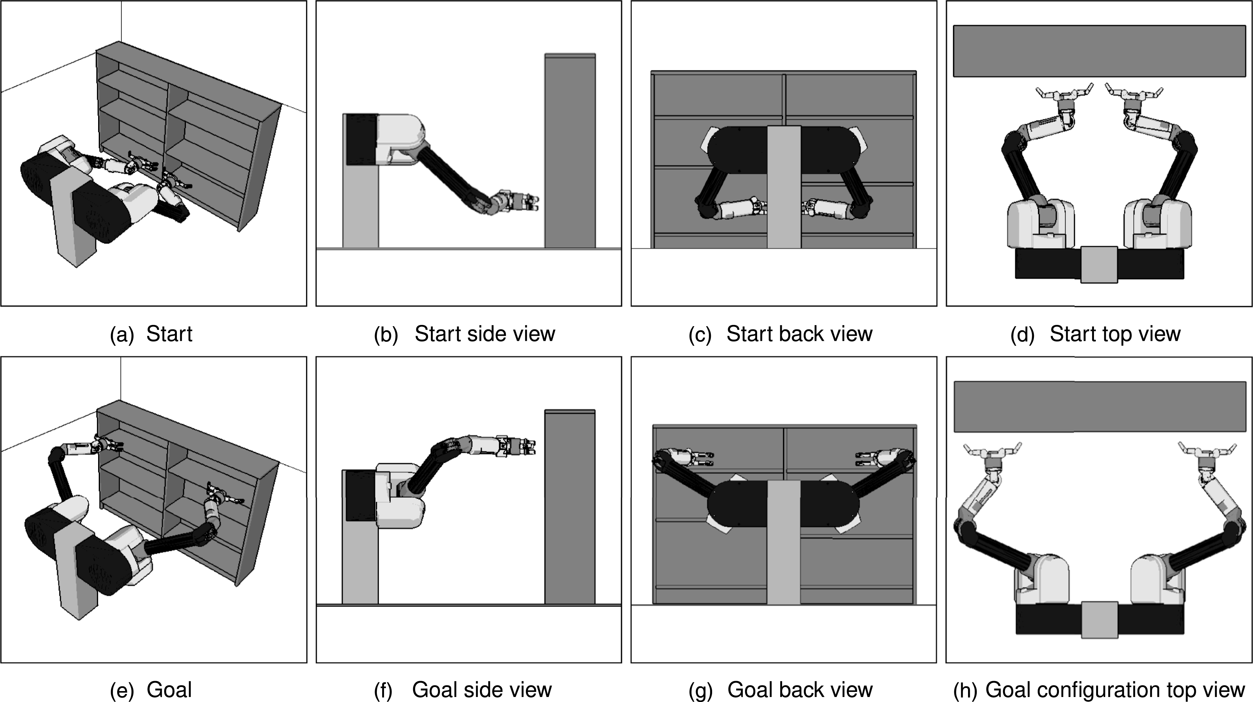

Figure 10 shows the performance of all algorithms when optimizing path length and obstacle clearance. When optimizing path length, AIT* performs similarly to BIT* and ABIT* which perform better than Lazy PRM* and EIT*, and find initial solutions nearly as fast as RRT-Connect and significantly faster than RRT* and LBT-RRT (Figure 10(a)). When optimizing obstacle clearance, AIT* and EIT* again outperform all tested asymptotically optimal planners but do not find initial solutions as fast as RRT-Connect, which still has a computational advantage because it does not calculate path cost (Figure 10(b)).

Figure 10.

This figure shows the planner performances on the dual-arm manipulator experiments described in Section 4.2.2 (Figure 9). The success plots show the percentages of successful runs over time. The cost plots show the median initial solution times and costs as squares and the median solution costs over time as thick lines, both with nonparametric 99% confidence intervals shown as error bars and shaded areas, respectively. Unsuccessful runs were taken as infinite costs. The results show when optimizing path length, AIT* performs nearly identically to BIT* and ABIT*, which all outperform Lazy PRM*, FMT*, and EIT*, and clearly outperform LBT-RRT and RRT* (a). When optimizing obstacle clearance, EIT* and AIT* outperform all other almost-surely asymptotically optimal planners (b).

4.3. Knee replacement dislocation problem

Calculating heuristics with an asymmetric bidirectional search can also improve performance on the feasible planning problem by guiding the search towards the goal. The knee replacement dislocation problem evaluates the potential of medial dislocation for the Oxford Domed Lateral Unicompartmental Knee Replacement (UKR; Pandit et al., 2010, Figure 11) ² by searching for a path to free the mobile bearing.

Figure 11.

A multiview illustration of the knee replacement dislocation experiment. The 3D model of the Oxford Domed Lateral UKR is reproduced from Figure 1 in Pandit et al. (2010) (a). The experiments presented in this paper used a simplified approximation of the Oxford Domed Lateral UKR (b). The start state of the mobile bearing is between the two fixed parts (b) with the search space and goal region shown as red and green regions, respectively (c). The goal region is the set of bearing positions in medial dislocation between the tibial and femoral components (d).

The Oxford Domed Lateral UKR consists of metal femoral and tibial components which are fixed to the bone and a mobile polyethylene bearing which separates the metal components (Gunther et al., 1996). Medial dislocation occurs when there is enough space between the tibial and femoral components for the mobile bearing to move onto the tibial-component wall where it may be trapped by the femoral component. The dislocation risk for different relative poses of the femoral and tibial components has been analyzed by using planning algorithms to search for paths that allow the bearing to reach a region representative of dislocation (Yang et al., 2020, 2021). Figures 11(b) and (c) respectively illustrate the start state and goal region of the mobile bearing and the fixed poses of the tibial and femoral components used in this experiment. The state space of this problem is   SE (3), and the mobile bearing is free to move and rotate in any direction not in collision with the fixed parts.

Figure 12 shows the performance of all planners when optimizing path length and obstacle clearance. When optimizing path length, EIT* outperforms all other tested planners. AIT* is the second best performing algorithm followed by FMT*, BIT*, and ABIT*. The OMPL implementations of LBT-RRT and RRT-Connect did not allow goals to be defined as a region and were replaced with RRT for this experiment. When optimizing obstacle clearance, EIT* again outperforms all other tested planners and is the only planner that achieved a success rate of 100%.

Figure 12.

The planner performances on the knee replacement dislocation problem described in Section 4.3 (Figure 11). The success plots show the percentages of successful runs over time. The cost plots show the median initial solution times and costs as squares and the median solution costs over time as thick lines, both with nonparametric 99% confidence intervals shown as error bars and shaded areas, respectively. Unsuccessful runs were taken as infinite costs. The results show that when optimizing path length, EIT* and AIT* outperform all other planners in terms of success rates, median initial solution times, and median solution quality over time. Lazy PRM* finds solutions as fast as EIT* for some random sequences of samples, but reaches the time limit before finding any solution for other random sequences. When optimizing obstacle clearance, EIT* again outperforms all other tested planners in terms of the above measures. RRT-Connect and LBT-RRT were not tested in this experiment, as their available OMPL implementations do not support goal regions.

5. Discussion

The experiments presented in Section 4 demonstrate the benefits of sampling-based path planning with an asymmetric bidirectional search. This section discusses the results of these experiments, elaborates on the algorithmic differences between AIT* and EIT*, and presents possible extensions to asymmetric bidirectional algorithms in sampling-based path planning and beyond.

Section 4 shows the performance of AIT*, EIT*, and eight other sampling-based algorithms on a diverse set of 12 problems optimizing two objectives. When optimizing path length, the experiments show that AIT* and EIT* are competitive to the other tested planners in terms of initial solution times, success rates, and solution quality over time.

When optimizing obstacle clearance, the experiments show that EIT* outperforms all other tested asymptotically optimal planners by finding initial solutions faster, reaching 100% success rates sooner, and providing the highest quality solution for most of the time. AIT* is often the second-best performing planner on this objective and even competitive to EIT* on the robotic arm experiments.

The batch size of AIT* and EIT* was kept constant for all presented experiments, while the performance of RRT-based planners was tuned to the problem dimension by adjusting the maximum edge length. This shows that AIT* and EIT* can perform well without problem-specific batch sizes but can also motivate future research to investigate advanced batch-size calculations, including variable and adaptive batch sizes.

The experiments presented in Section 4 keep the collision detection resolution constant within each problem. This resolution determines the false-negative collision rate, i.e., the percentage of edges that are considered valid but in reality are not. What is considered an acceptable false negative collision rate depends on the application of the planning algorithm. Experiments not presented in this paper showed that the relative performance of AIT* and EIT* compared to other algorithms improves as edge evaluation becomes more computationally expensive, e.g., due to finer collision detection resolution or more complex analysis. This may be because AIT* and EIT* often fully evaluate fewer edges than other algorithms and their performance is therefore not as sensitive to the collision detection resolution. If edge evaluation is computationally inexpensive, e.g., due to coarse collision detection resolution, then the benefits of the accurate heuristics calculated in AIT* and EIT* may not justify the computational cost required to calculate them and other sampling-based planners may perform better in these cases.

Edge evaluation is also computationally expensive for systems with kinodynamic constraints, when full edge evaluation requires solving a two-point Boundary Value Problem (BVP). The accurate heuristics calculated by AIT* and EIT* can reduce the number of BVP solved, but AIT* and EIT* require exact solutions to the BVPs. Other almost-surely asymptotically optimal algorithms do not require exact BVP solutions even for problems with kinodynamic constraints (Hauser and Zhou 2016; Li et al., 2016; Kleinbort et al., 2020a; Shome and Kavraki 2021).

AIT* and EIT* use different algorithms for the reverse and forward searches of their asymmetric bidirectional search (Table 1). The change in forward search algorithms from A* in AIT* to AEES in EIT* is motivated by the benefits of effort heuristics, which cannot be exploited with A*, and justify the computational overhead induced by the increased complexity of AEES. The change in reverse search algorithms from LPA* in AIT* to A* in EIT* is motivated by the observations that repairing the reverse search tree with LPA* is only more efficient than restarting A* for small changes in the search tree (between 1% and 2%; Table 1, Aine and Likhachev 2016), and that detecting invalid edges with the forward search often results in larger changes in the reverse search tree. Implementing increasingly dense collision detection in an LPA* reverse search would additionally require either further bookkeeping to keep track of which portion of the tree was checked with which resolution or result in duplicated collision detection effort on some of the edges.

The presented asymmetric bidirectional approach in which two searches inform each other with complementary information can potentially be beneficial in all problem domains where full edge evaluation is computationally expensive, e.g., because of computationally expensive true edge cost computation or complex collision detection. If this edge cost computation can inexpensively be approximated by a heuristic, then the reverse search can combine such heuristics between multiple states into more accurate heuristics between each state and the goal, similar to AIT* and EIT*.

6. Conclusion

Informed path planning algorithms can use problem-specific knowledge in the form of heuristics to improve their performance, but selecting appropriate heuristics is difficult. This is because heuristics are most effective when they are both accurate and computationally inexpensive to evaluate, which are often conflicting characteristics. Many informed planners additionally can only use problem-specific knowledge if it is expressible as admissible heuristics, which is not always possible for all optimization objectives.

This paper presents two almost-surely asymptotically optimal path planning algorithms that address these challenges by using asymmetric bidirectional searches that simultaneously calculate and exploit accurate, problem-specific heuristics. AIT* uses an inexpensive reverse search to combine admissible a priori cost heuristics between two states into a more accurate but still admissible cost heuristic between each state and the goal. This heuristic is exploited to make AIT*’s forward search more efficient and repaired whenever the forward search detects that it uses invalid edges. In this way, information is passed between both directions of the bidirectional search, as each search informs the other.

EIT* builds on AIT* by additionally calculating inadmissible cost and effort heuristics with its reverse search. This additional knowledge about the computational effort to validate a path can be calculated for any optimization objective and exploited by EIT*’s forward search to order its search in a solution-oriented manner. This improves anytime performance when the cost of a path does not correlate well with the computational effort required to validate it and allows EIT* to find initial solutions quickly, even if an admissible cost heuristic is not available for an optimization objective.

The benefits of simultaneously calculating and exploiting ever more accurate heuristics through an asymmetric bidirectional search are demonstrated on 12 diverse problems in abstract, robotic, and biomedical domains. EIT* outperforms all other tested asymptotically optimal planners when optimizing obstacle clearance and performs competitively when optimizing path length. AIT* is often the second best performing asymptotically optimal planner when optimizing obstacle clearance and also performs competitively when optimizing path length.

Information on the OMPL implementations of AIT* and EIT* as well as the software framework for running the experiments and creating the corresponding plots will be available at https://robotic-esp.com/code/.

Supplemental Material

Supplemental Material

Supplemental Material