IHSCR: Energy-efficient clustering and routing for wireless sensor networks based on harmony search algorithm

Abstract

Clustering and routing are two key techniques to improve the energy efficiency of wireless sensor networks. As clustering and routing for improving the energy efficiency of wireless sensor networks are NP-hard problems, increasing meta-heuristic algorithms are introduced for solving them. However, due to their discreteness and strong constraints, most meta-heuristics are unsuitable or inefficient to optimize them. Harmony search algorithm is one of the most suitable meta-heuristics for solving these problems. This article proposes a new energy-efficient clustering and routing algorithm based on harmony search algorithm to improve the energy efficiency of wireless sensor networks. The proposed approach contains two parts: clustering phase and routing phase. First, a new objective function model, which has considered balancing the energy consumption of both gateways and regular nodes as well as considered routing, is established for the clustering phase. Then, a new energy-efficient clustering algorithm is designed based on several improvements made to harmony search algorithm: (1) a discrete encoding scheme of a harmony for clustering is proposed; (2) a roulette wheel selection method is designed to choose a gateway for a regular sensor node to join, which is employed by two steps (i.e. initialization of harmony and improvisation of a new harmony); (3) the dynamically changed harmony memory considering rate is designed for improvisation of a new harmony; (4) a local search scheme is proposed to improve the best harmony within the harmony memory in iterations. In addition, the improved harmony search based energy-efficient routing algorithm that we proposed previously is employed to balance the energy consumption of gateways in the routing phase. The proposed approach is compared with several popular meta-heuristic-based clustering algorithms over extensive wireless sensor networks cases. The experimental results clearly demonstrate the superiority of the proposed approach.

Introduction

Wireless sensor networks, 1 of the 10 emerging technologies, ¹ are the core technology of the Internet of Things (IoT) and will change the world. ² As micro-electro-mechanical system (MEMS) and wireless communication technology have achieved rapid progress, ³ wireless sensor network (WSN) has developed dramatically in recent years. It has been widely applied in different fields, and then, it is changing the human life profoundly. The wide applications of WSNs include military sensing, ⁴ intelligent agriculture, ⁵ mobile target detection water, ⁶ health monitoring, ⁷ smart grid, ⁸ human activity monitoring, ⁹ and so on.

A WSN comprises of a large number of sensor nodes, which contain sensing, computing, communication, and power supply components that provide an opportunity to monitor and control the physical world. As the sensor nodes used in most applications are powered by batteries, the research on the improvements of energy efficiency of WSNs, to extend the network lifetime as far as possible, is still the focus at present and in the future. There are lots of schemes which have been proposed for this purpose, such as “low-power radio communication hardware,” ¹⁰ and “energy-aware medium access control (MAC) layer protocols.”^11,12 However, clustering is one of the most effective techniques for saving the energy of sensor nodes. In a cluster-based WSNs, the network comprises of several groups called clusters, in each of which there is a unique node known as cluster head (CH) takes charge of its cluster. In a cluster, all the member sensor nodes sense local data and transmit them to the CH, and then, the CH aggregates the local data and finally sends the aggregated data to the base station (BS) directly or via other CHs. Therefore, it can avoid transmitting high volumes of redundant data from each sensor node to the BS, so as to reduce the energy consumption of the whole network.

In many WSNs, as the CHs are selected usually from the regular sensor nodes, they may run out of energy quickly for receiving data from member sensor nodes, aggregating the local data, and transmitting data to the BS frequently. Thus, many researchers have introduced some special nodes called gateways or relay nodes,^13–15 with much more energy than the regular nodes, to be CHs all the time. In this article, such gateways are also employed. Because the gateways are also battery powered, and the gateways and the regular nodes may not be uniformly deployed in a sensing area, it is important to assign the regular nodes to the gateways properly. Otherwise, some gateways may die quickly as they are overloaded with excessive member regular nodes. For balancing the energy consumption of gateways, some regular nodes may be assigned to the farther gateways rather than their nearest gateways. Thus, those regular nodes that are assigned to the far away gateways will run out of energy quickly due to long haul transmission and finally lose the ability of sensing their local information. Therefore, for prolonging the whole network lifetime, the assignment of regular nodes to gateways, obtained by clustering algorithm, should consider not only the energy consumption of CHs but also the energy consumption of regular nodes. It is worth noting that for a WSN with $n$ regular nodes and $m$ gateways, the number of possible clusters (solutions) is $m^n$ , which means that it is scarcely possible for a brute force approach to find out the optimal clustering solution of a large-scale WSN. ³ Instead, it is feasible and reasonable to design meta-heuristic-based clustering algorithms for calculating as good as possible a solution in a certain period of time.

In this article, for a WSN with $n$ regular nodes and $m$ gateways, the problems to be addressed are calculating as good as possible a solution of assignment of regular nodes to gateways in the clustering phase and computing as good as possible a forwarding path for each gateway in the routing phase, so that maximizing the whole network lifetime as far as possible. Harmony search (HS) algorithm is one of the most suitable meta-heuristics for solving this type of clustering problem in this article, because its discrete encoding scheme and the generation method of a new solution designed for this problem can reduce the search space, thus, contribute to find as good as possible a solution and improve the convergence speed. So far, the research of applying HS algorithm to solve this type of clustering problem of WSNs is few. This article tries to develop an energy-efficient clustering algorithm for WSNs based on HS algorithm, called improved harmony search based clustering and routing (IHSCR) algorithm. It is worth noting that in the routing phase, the improved harmony search based energy-efficient routing (IHSBEER) algorithm that we developed in Zeng and Dong ¹⁶ is employed. Therefore, the proposed approach in this article is called IHSCR algorithm.

The main contributions of this article are shown as follows:

1. A new energy-efficient clustering algorithm called improved harmony search based clustering (IHSC) for dealing with the clustering problem of WSNs is developed based on several improvements made to the traditional HS algorithm.

2. IHSBEER algorithm is employed by IHSCR to balance the energy consumption of gateways in the routing phase.

3. The proposed IHSCR performs far better than other clustering algorithms over balance of the energy consumption of sensor nodes (especially the regular nodes), which has considerable contribution on improving the energy efficiency of WSNs and extending the whole network lifetime.

The rest of this article is organized as follows. Section “Related works” describes the related works. The mathematical model, containing the system model and the proposed objective function model, is presented in section “Mathematical model.” Section “IHSCR algorithm” first introduces the HS algorithm briefly, and then, the proposed approach is described in sufficient detail. The experimental results and analysis to evaluate the proposed approach are presented in section “Experimental results and analysis.” Section “Conclusion and future works” summarizes this article and advances further work.

Related works

At present, a large amount of research is devoted to the design and development of clustering algorithm for WSNs. In this section, a brief overview of the clustering algorithms, especially the meta-heuristic-based clustering algorithms of WSNs, is presented. More references and discussions about this topic can be viewed in the literatures.^17–21

Energy-efficient load-balanced clustering algorithm (EELBCA) was proposed by Kuila and Jana ¹⁴ to address energy efficiency and load balancing of WSNs. In the clustering phase, a min-heap containing the CHs is built in the order of smallest to largest in number of sensor nodes assigned to the CHs. When there were unassigned sensor nodes, the sensor node, which is nearest to the root node of the min-heap among the unassigned sensor nodes, is assigned to the root node of the min-heap. Then, adjusting the min-heap to keep the minimum loaded gateway at root. Continue the above process until all the sensor nodes are assigned to CHs. For $n$ sensor nodes and $m$ CHs, the time complexity of EELBCA is O (n log m). In EELBCA, the residual energy of CHs and regular nodes are not considered. The experimental results show that EELBCA outperforms greedy load-balanced clustering algorithm (GLBCA) ²² and LBC ²³ in terms of energy efficiency, load balancing, the number of dead sensor nodes, and execution time.

Yi et al. ²⁴ proposed a power-efficient and adaptive clustering hierarchy (PEACH) protocol to reduce the energy consumption of sensor nodes and prolong the network lifetime, by forming clusters without additional overhead on CHs selection and supporting adaptive multi-level clustering. When forming clusters, PEACH protocol does not require overhead of transmitting packets for advertising and announcing CHs, joining the clusters, and scheduling of intra-cluster communication, compared with the existing clustering algorithms. What is more, PEACH protocol supports both the location-aware WSNs and the location-unaware WSNs. As PEACH protocol supports adaptive multi-level clustering, it is less affected by the size of sensing field or the distribution of sensor nodes. The experimental results show that PEACH protocol performs better than other clustering algorithms compared in terms of energy consumption and network lifetime.

Jin et al. ²⁵ proposed an energy-efficient multi-level clustering (EEMC) algorithm to improve the energy efficiency of WSNs. The data transmission operation in this algorithm is also divided into rounds. Each round begins with the cluster setup phase and then followed by the data transmission phase. In the cluster setup phase, first, the optimal expected number of cluster levels and the number of sensor nodes in each level are obtained by EEMC algorithm. Then, EEMC algorithm assigns the sensor nodes to their own clusters and elects CH for each cluster at the same time. As the rounds of data transmission operation increase, the optimal number of cluster levels and CHs will be found asymptotically. The experimental results demonstrate that EEMC algorithm performs better than low energy adaptive clustering hierarchy (LEACH) ²⁶ and energy-efficient multi-level k-hop (EEMK) in terms of network lifetime and transmission latency. Especially, when the path loss exponent is 2, EEMC algorithm could get minimum latency.

GLBCA was proposed by Low et al. ²² to address the load-balanced clustering problem (LBCP) by assigning regular nodes to gateways, so as to distribute the traffic load among the gateways for assuring no gateway is overloaded in WSNs. GLBCA utilizes an approximation algorithm for this non-deterministic polynomial (NP)-hard problem, which is able to guarantee a performance ratio of 3/2. However, GLBCA does not take into consideration the residual energy of both regular nodes and CHs.

Genetic algorithm (GA)-based load-balanced clustering algorithm was proposed by Kuila et al. ¹⁵ to address the LBCP for WSNs. In this algorithm, each chromosome represents a complete assignment of all the regular nodes to their corresponding gateways. A fitness function that considers not only minimizing the maximum load of a gateway but also concentrating on the load distribution among all the gateways is built. However, the residual energy of both the CHs and the regular nodes is not taken into consideration. The experimental results indicate that this algorithm is better than simple GA, LBC and the least distance clustering (LDC), ²⁷ and so on, in terms of load balancing of the gateways for equal or unequal load of the regular nodes as well as energy consumption, number of active regular nodes, and execution time.

Latiff et al. ²⁸ proposed an energy-aware particle swarm optimization clustering (PSO-C) algorithm for WSNs using PSO. In PSO-C, each particle represents a CHs selection solution. A fitness function considering both the intra-cluster distance and the residual energy of CH candidates is defined. PSO-C assumes that the data are transmitted from CHs to the BS by single hop instead of multi-hop. The simulation results indicate that PSO-C performs better than LEACH and LEACH-centralized (LEACH-C) in terms of data delivery and network lifetime.

Fuzzy energy-aware unequal clustering (EAUCF) algorithm was proposed by Bagci and Yazici ²⁹ to address the hot spots problem of WSNs. In EAUCF, a fuzzy logic approach, which employs two fuzzy input variables that are the distance to the BS and the residual energy, is adopted to calculate competition radius of each tentative CH. With this fuzzy logic approach, if a tentative CH is closer to the BS or had lower residual energy than another, it will get a smaller competition radius. The CH competition begins after all the tentative CHs have determined their competition radius. Each tentative CH advertises a message, which includes node ID, competition radius, and the residual energy of the source node, to compete with other tentative CHs within its competition range. If the residual energy of a tentative CH is the highest among the tentative CHs which it receives message from, then it becomes a CH. Thus, the intra-cluster work of the CHs, which either are close to the BS or have low residual energy, is decreased. On real WSNs, some CHs elected by EAUCF are likely to be isolated nodes. The experimental results show that EAUCF outperforms LEACH, cluster-head election mechanism using fuzzy logic (CHEF), and energy-efficient unequal clustering (EEUC), in terms of three metrics, that is, first node dies, half of the nodes alive, and energy efficiency, in all scenarios.

Kuila and Jana ³ proposed a differential evolution–based clustering algorithm (DECA) to prolong the network lifetime by reducing energy consumption of highly loaded CHs. In this clustering algorithm, an efficient encoding and decoding scheme of the solution vector is proposed to enable each solution vector to represent the complete assignment of regular nodes to gateways, which is the key step to applying DE algorithm to design clustering algorithm for WSNs. And a fitness function that has considered the energy consumption of both gateways and regular nodes is proposed also, which has a great contribution to the extension of all nodes’ lifetime. What is more, a local improvement phase was proposed to improve the quality of the trial vector. DECA assumes that the gateways communicate with the BS directly. The experimental results indicate that DECA outperforms the traditional DE, GA, load-balanced clustering (LBC), GLBCA, and EELBCA, in terms of energy consumption, network lifetime, and number of dead regular nodes.

Lots of existing clustering algorithms have not considered the residual energy of the sensor nodes. In addition, most of them have not employed multi-hop communication between the CHs and the BS. Therefore, the sensor nodes with low energy, especially those CHs far away from the BS, would run out of energy quickly, which would shorten the whole network lifetime. The proposed IHSCR algorithm in this article is to extend the whole network lifetime as far as possible by balancing the energy consumption of both gateways and regular nodes. In the clustering phase, we have taken the residual energy of gateways into consideration. And the standard deviation of distance from all the regular nodes to their gateways is minimized, so the energy consumption of regular nodes is balanced. In routing phase, we have adopted multi-hop communication between the gateways and the BS, by employing the routing algorithm IHSBEER that we proposed in Zeng and Dong, ¹⁶ so as to balance the energy consumption of gateways in the transmission phase.

Mathematical model

This section first presents the system model, containing the energy consumption model and the network model, employed by the proposed IHSCR algorithm. Then, an effective objective function of the clustering problem optimized in this article is proposed.

System model

Energy consumption model

The radio model in Heinzelman et al. ²⁶ is used to estimate the energy consumption of wireless communication in this article. This model utilizes free space or multipath fading channels according to the distance between the transmitting node and the receiving node. If the distance is less than a threshold $d_0$ , the free space (fs) model will be employed; otherwise, the multipath (mp) model will be used. Therefore, to transmit a k-bits message in d-meters, the radio consumes energy as follows

$$E_{\mathrm{Tx}}(k,d)=\{\begin{array}{cc}{E}_{\mathrm{elec}}*k+{\epsilon }_{\mathrm{fs}}*k*d^2\hfill & \mathrm{for}d<d_0\hfill \\ \multicolumn{1}{c}{E_{\mathrm{elec}}*k+{\epsilon }_{\mathrm{mp}}*k*d^4}& \mathrm{for}d\ge d_0\hfill \end{array}$$ (1)

where $E_{\mathrm{elec}}$ denotes the unit energy consumption of electronic circuit; ${\epsilon }_{\mathrm{fs}}$ and ${\epsilon }_{\mathrm{mp}}$ represent the unit energy consumption in free space and multipath fading channels, respectively.

The energy required for the radio to receive a k-bits message is shown as follows

$$E_{\mathrm{Rx}}\left(k\right)=E_{\mathrm{elec}}*k$$ (2)

Network model

If a gateway is within the communication range of a regular node, the regular node can be assigned to the gateway. In our assumed WSN model, all the regular nodes and gateways are deployed randomly in the scenario, and the communication range of any regular node must cover at least one gateway and any gateway must have at least one forwarding path to the BS. Once the regular nodes and gateways are deployed, they remain stationary. In our approach, the operation of data aggregation is also divided into rounds similar to LEACH algorithm. ²⁶ In each round, all the regular nodes sense the local environmental information, process them into useful data packets, and send the packets to their CHs using carrier sense multiple access/collision avoidance (CSMA/CA) MAC protocol. ³⁰ Then, each CH aggregates the data packets to discard the redundant and uncorrelated data and transmits the aggregated data packets to the BS via multi-hop communication also using CSMA/CA MAC protocol.

Objective function

This article is aimed at maximizing the whole network lifetime via energy-efficient clustering and routing techniques. In the clustering phase, the problem to be addressed is calculating as good as possible a solution of assignment of regular nodes to gateways, so as to balance the energy consumption of both gateways and regular nodes. For balancing the energy consumption of gateways, we introduce the concept of gateway lifetime ³ as follows

$$L\left(g_i\right)=\frac{E_r\left(g_i\right)}{E_c\left(g_i\right)}$$ (3)

where $L\left(g_i\right)$ is the lifetime of the gateway $g_i$ , $E_r\left(g_i\right)$ denotes the residual energy of $g_i$ , and $E_c\left(g_i\right)$ denotes the total energy consumption of $g_i$ in a single round. From equation (3), we can see that the lifetime of a gateway with lower residual energy will be extended if it consumes less energy in a single round. Here, $E_c\left(g_i\right)$ can be formulated as shown in equation (4), which is different from that in Kuila and Jana ³

$$E_c\left(g_i\right)=n_i\times E_{\mathrm{Rx}}\left(k\right)+n_i\times E_{\mathrm{DA}}\left(k\right)+E_{\mathrm{Tx}}(l,d_{g_i,N_i})$$ (4)

where $n_i$ denotes the number of member regular nodes of $g_i$ . $E_{\mathrm{DA}}(k)$ represents the energy required to aggregate k-bit message, where $E_{\mathrm{DA}}(k)=E_{\mathrm{da}}*k$ ; $E_{\mathrm{da}}$ is the unit energy consumption to aggregate message. $l$ denotes the size of packets that $g_i$ needs to send to the BS. Because the next hop of $g_i$ is determined by the routing algorithm, here, the gateway $N_i$ called the default next hop of $g_i$ is utilized to temporarily represent the next hop of $g_i$ for calculating $E_c(g_i)$ . In our approaches, $N_i$ is specified as the gateway which is closer to the BS than $g_i$ and is closer to $g_i$ than other gateways, while the next hop of $g_i$ is always the BS in Kuila and Jana. ³ Once $N_i$ has run out of energy, $g_i$ need to recalculate the default next hop. Obviously, it can be seen from equation (4) that the less member regular nodes a gateway has, the less energy it will consume in a single round. Therefore, if a gateway with lower residual energy contains less member regular nodes, its lifetime will be extended.

It is obvious that the smaller the standard deviation ( ${\sigma }_L$ shown in equation (5)) of lifetime of the gateways, the higher the level of balancing the energy consumption of gateways, ²² so the gateways will survive for almost the same time

$${\sigma }_L=\sqrt{\frac{1}{m}*\sum _{i=1}^m{({\mu }_L-L\left(g_i\right))}^2}$$ (5)

where $m$ is the number of gateways and ${\mu }_L$ is the mean of lifetime of all the gateways, ${\mu }_L=1/m\sum _{i=1}^{m}L(g_i)$ .

To prolong the whole network lifetime, we not only need to balance the energy consumption of gateways, but also need to keep balance between the energy consumption of regular nodes as far as possible. Because the environmental information cannot be collected if the corresponding regular nodes run out of energy. From equation (1), we can see that when the size ( $k$ ) of the packets need to be send is constant, the farther the transmission distance ( $d$ ) is, the more energy a node will consume. In this article, the size of the packets that regular nodes send to gateways is equal. Thus, the energy consumption of regular nodes can achieve a balance only if the standard deviation $\left({\sigma }_D\right)$ of the distance from all the regular nodes to their gateways is reduced as far as possible, which is more reasonable than that in Kuila and Jana ³ where the energy consumption of regular nodes is balanced by minimizing the standard deviation of the cluster distance of all the clusters. Because though the standard deviation of the cluster distance is small, the difference between the distance from some regular nodes to their gateways in some clusters may be relatively large, which has a negative effect on the balance of the energy consumption of regular nodes. In this article, ${\sigma }_D$ , that is, the standard deviation of the distance from all the regular nodes to their gateways, is formulated as follows

$${\sigma }_D=\sqrt{\frac{1}{n}*\sum _{i=1}^n{({\mu }_D-D\left(r_i\right))}^2}$$ (6)

where $n$ is the number of alive regular nodes, $D\left(r_i\right)$ denotes the distance from $r_i$ to its gateway, and ${\mu }_D$ is the mean of distance from all the regular nodes to their gateways, ${\mu }_D=1/n\sum _{i=1}^{n}D(r_i)$ .

Based on above, we establish the fitness function as shown in equation (7), which has considered the balance of the energy consumption of both gateways and regular nodes, and can adjust their weights in the meantime

$$f={\omega }_1{\sigma }_L+{\omega }_2{\sigma }_D$$ (7)

where ${\omega }_1$ and ${\omega }_2$ are the weight factors of ${\sigma }_L$ and ${\sigma }_D$ , respectively. They all take values between 0 and 1, and ${\omega }_1+{\omega }_2=1$ .

IHSCR algorithm

This section first introduces the HS algorithm briefly. Then, the implementation of IHSCR algorithm is described in sufficient detail.

HS algorithm

HS algorithm, a meta-heuristic, is first developed by Geem et al., ³¹ which is inspired by the process of looking for a perfect state of harmony when musicians improvising. The HS algorithm has a simple concept and is easy to implement. What is more, it has strong global search ability, according to lots of research. So far, HS algorithm has been employed by many researchers to solve various real-world optimization problems. For instance, Ser et al. ³² proposed HS-based centralized and distributed spectrum allocation techniques to solve the spectrum channel assignment problem in cognitive wireless networks. Manjarres et al. ³³ proposed a two-objective localization approach based on the combination of the HS algorithm and a local search procedure to deal with the localization problem in WSNs. Yi et al. ³⁴ introduced a parallel chaotic local search scheme into the HS algorithm for solving the engineering design optimization problem. Chatterjee et al. ³⁵ proposed an opposition-based HS algorithm via introducing opposition-based learning technique into the HS algorithm, to solve the combined economic and emission dispatch problems of power systems. Kulluk et al. ³⁶ introduced the HS algorithm for the supervised training of feed-forward type training neural networks, which are used to solve the classification problems. Yi et al. ³⁷ proposed a nested maximin Latin hypercube design approach based on the combination of successive local enumeration and a modified global HS algorithm, for the design of computer experiments.

The five steps of the original HS algorithm are shown as follows: ³⁸ (1) initialization of the optimization problem and parameters; (2) initialization of the harmony memory (HM); (3) improvisation of a new harmony; (4) update the HM; and (5) repeat steps 3 and step 4 until the stopping criterion is satisfied:

• 1. Initialization of the optimization problem and parameters

First, the optimization problem is formulated as follows

$$\mathrm{Minimize}f\left(\mathbf{X}\right)\mathrm{s}.\mathrm{t}.x_i\in {\mathbf{X}}^i,i=1,2,\dots ,n$$ (8)

where $\mathbf{X}$ is the set of design variables; $f(\mathbf{X})$ is the objective function; ${\mathbf{X}}^i$ is the set of the possible values of $x_i$ , when the problem belongs to continuous optimization problem, ${\mathbf{X}}^i=\{x_i|x_i^L\le x_i\le x_i^U\}$ , where $x_i^L$ and $x_i^U$ are the lower and upper bounds of $x_i$ , respectively; and $n$ is the number of design variables.

This step also has specified the parameters of HS algorithm: the harmony memory size (HMS) which is the number of solution vectors in the HM and usually set to 5, harmony memory considering rate (HMCR), pitch adjusting rate (PAR), bandwidth (bw), and stopping criterion (maximum iteration number). Here, HMCR, PAR, and bw are used to explore better solution vectors and both defined in step 3.

• 2. Initialization of the HM

The HM, as shown in equation (9), is a memory space where store the solution vectors called harmonies that are randomly generated using uniform distribution

$$\mathrm{HM}=\left[\begin{array}{c}{\mathbf{X}}_1\\ {\mathbf{X}}_2\\ ⋮\\ {\mathbf{X}}_i\\ ⋮\\ {\mathbf{X}}_{\mathrm{HMS}}\end{array}\right]=\left[\begin{array}{cccccc}{x}_{1,1}& x_{1,2}& \cdots & x_{1,j}& \cdots & x_{1,n}\\ x_{2,1}& x_{2,2}& \cdots & x_{2,j}& \cdots & x_{2,n}\\ ⋮& ⋮& ⋮& ⋮& ⋮& ⋮\\ x_{i,1}& x_{i,2}& \cdots & x_{i\mathrm{,}j}& \cdots & x_{i\mathrm{,}n}\\ ⋮& ⋮& ⋮& ⋮& ⋮& ⋮\\ x_{\mathrm{HMS},1}& x_{\mathrm{HMS},2}& \cdots & x_{\mathrm{HMS}\mathrm{,}j}& \cdots & x_{\mathrm{HMS}\mathrm{,}n}\end{array}\right]$$ (9)

• 3. Improvisation of a new harmony

A new harmony, $\mathbf{X}\prime =(x_1\prime ,x_2\prime ,\dots x_i\prime ,\dots ,x_n\prime )$ , is generated through two steps: harmony memory considerations and pitch adjustments. The first step is shown as follows

$$x{\prime }_i\leftarrow \{\begin{array}{cc}{x}_i\prime \in \{x_{1,i},x_{2,i},\dots ,x_{\mathrm{HMS},i}\}\hfill & \mathrm{if}(P_1<\mathrm{HMCR})\hfill \\ \multicolumn{1}{c}{x_i\prime \in {\mathbf{X}}^i}& \mathrm{else}\hfill \end{array}$$ (10)

where HMCR is a constant between 0 and 1, and $P_1$ is a random number generated from 0 to 1. Equation (10) means that $x{\prime }_i$ should be selected from the ith column of HM, that is, $\{x_{1,i},x_{2,i},\dots ,x_{\mathrm{HMS},i}\}$ if $P_1$ is smaller than HMCR; otherwise, $x{\prime }_i$ can be a feasible value belonging to ${\mathbf{X}}^i$ .

Those elements of the new harmony, which are selected from the HM, need to be determined whether it should be pitch-adjusted. This step is shown as follows

$$\mathrm{Pitch}\mathrm{adjusting}\mathrm{decision}\mathrm{for}x{\prime }_i\leftarrow \{\begin{array}{c}\mathrm{Yes}\hfill \\ \multicolumn{1}{c}{\mathrm{No}}\end{array}\begin{array}{c}\mathrm{if}(P_2<\mathrm{PAR})\hfill \\ \multicolumn{1}{c}{\mathrm{else}}\end{array}$$ (11)

where PAR is a constant between 0 and 1, and $P_2$ is a random number generated from 0 to 1. Equation (11) means that if $P_2$ is smaller than PAR, $x{\prime }_i$ needs to be adjusted; otherwise, it remains unchanged. If the decision of equation (11) is “Yes,” the adjustment process of $x{\prime }_i$ is shown as follows

$$x{\prime }_i\leftarrow x{\prime }_i\pm \mathrm{rand}*\mathrm{bw}$$ (12)

where bw is an arbitrary distance bandwidth, and $\mathrm{rand}$ is a random number generated between 0 and 1 using uniform distribution.

• 4. Update the HM

If the new harmony, that is, $\mathbf{X}\prime =(x_1\prime ,x_2\prime ,\cdots ,x_i\prime ,\cdots ,x_n\prime )$ , is better (judged by fitness) than the worst harmony in the HM, replace the existing worst harmony with the new harmony.

• 5. Repeat steps 3 and step 4 until the stopping criterion is satisfied

If the stopping criterion is satisfied, the computations are terminated; otherwise, repeat steps 3 and 4.

The proposed approach

There are two phases, that is, clustering phase and routing phase, in our proposed approach IHSCR. First, the network should be setup before performing the proposed approach, like other clustering approaches.^14,15,22 During the network setup process, all the gateways and regular nodes are assigned unique IDs. Then each regular node broadcasts a packet containing its ID to its neighbor nodes. Thereby, those gateways within its communication range are able to get its ID. After all the regular nodes have finished broadcasting, the gateways send the packets containing the local network information to the BS. Therefore, the gateways within the communication range of each regular node can be obtained by the BS. In the clustering phase, the proposed clustering algorithm, that is, IHSC algorithm, is executed by the BS to calculate the optimal clustering result. Then, the BS broadcasts the packets containing the optimal assignment of each regular node to the gateways, and the gateways broadcast the packets containing their IDs to their member regular nodes, so as to finish the clustering process. When a regular node has detected environmental information, it processes them to packet and sends the packet to its gateway. Then, the gateways aggregate the intra-cluster data. In the routing phase, the routing algorithm IHSBEER that we proposed in Zeng and Dong ¹⁶ is conducted by the BS to calculate optimal forwarding paths for gateways. Each gateway has stored the optimal forwarding path received from the BS and sends the aggregated data to the BS via multi-hop communication according to the forwarding path stored in its memory. Once any gateway or regular node runs out of energy, the network would require re-clustering.

Clustering algorithm

First, we propose a harmony search based clustering (HSC) algorithm for WSNs. Then, several improvements are made to the HS algorithm based on the characteristics of the clustering problem in this article, so that an IHSC algorithm is proposed. It is worth noting that the fitness function is the same as the objective function proposed in section “Objective function.”

Harmony search based clustering algorithm

Before applying HS algorithm to design clustering algorithm for the WSNs in this article, the following problems need to be addressed. First, how to encode a harmony matching with the clustering problem in this article? Then, how to improvise a new harmony? After these problems have been solved, the harmony search based clustering algorithm is proposed, and its flowchart is demonstrated in Figure 1.

Figure 1.

Flowchart of HSC algorithm.

• Encoding of harmony. As the purpose of the clustering algorithm in this article is to prolong the whole network lifetime by assigning the regular nodes to the gateways properly, the most effective encoding scheme of harmony is that each harmony (i.e. solution) in the HM denotes the complete assignment of all the regular nodes to the gateways. We adopt the following vector for representing the ith harmony in the HM

$${\mathbf{X}}_i=(x_{i,1},x_{i,2},\dots ,x_{i,j},\dots ,x_{i,n})$$ (13)

where ${\mathbf{X}}_i$ denotes the ith harmony of HM, $n$ is the number of alive regular nodes, and $x_{i,j}$ is the jth pitch of harmony ${\mathbf{X}}_i$ and maps the assignment of the regular node $r_j$ to a gateway. Here, the value of $x_{i,j}$ is the serial number of the gateway that regular node $r_j$ has joined. This discrete encoding method can make great contribution to reduce the search space.

For example, as we can see from Figure 2, the WSN scenario contains 5 gateways and 12 regular nodes, that is, the gateways set G = {g₁, g₂, g₃, g₄, g₅} and the regular nodes set R = {r₁, r₂, r₃, r₄, r₅, r₆, r₇, r₈, r₉, r₁₀, r₁₁, r₁₂}. Thus, the dimension of harmony in the HM is equal to the number of regular nodes, that is, n = 12. The edges between the regular nodes and the gateways mean that those regular nodes can communicate with those gateways connected by the edges, that is, those gateways are within the communication range of the regular nodes. Supposing the ith harmony X _i  = (2, 3, 4, 2, 3, 5, 1, 3, 1, 4, 5, 5), which means that regular node $r_1$ joins gateway $g_2$ , $r_2$ joins $g_3$ , and so on.

Figure 2.

A wireless sensor network with gateways.

For the convenience of describing the initialization procedure of harmony, we provide the following definition.

Definition 1

$\mathbf{CrGates}(r_i)$ : the set of gateways which are within the communication range of node $r_i$ . With the encoding scheme, we can randomly select a gateway in $\mathbf{CrGates}(r_i)$ to assign its serial number to the ith element of a harmony (i.e. the regular node $r_i$ joins that gateway), for initializing the ith element. After each element of the harmony has been assigned the serial number of a gateway, that is, all the regular nodes have joined their gateways, the harmony is initialized.

• Improvisation of a new harmony. Like the traditional HS algorithm, the improvisation of a new harmony in HSC algorithm is also based on two steps: harmony memory considerations and pitch adjustments. Supposing a new harmony is denoted by $\mathbf{X}\prime =(x{\prime }_1,x{\prime }_2,\dots ,x{\prime }_i,\dots ,x{\prime }_n)$ ; first, the element $x{\prime }_i$ of $\mathbf{X}\prime$ is generated by memory considerations as follows

$$x{\prime }_i\leftarrow \{\begin{array}{cc}{x}_i\prime \underset{\mathrm{rd}}{\to }\{x_{1,i},x_{2,i},\cdots ,x_{\mathrm{HMS},i}\}\hfill & \mathrm{if}(P_1<\mathrm{HMCR})\hfill \\ \multicolumn{1}{c}{x_i\prime \underset{\mathrm{rd}}{\to }\mathbf{CrGates}\left(r_i\right)}& \mathrm{otherwise}\hfill \end{array}$$ (14)

where $\underset{\mathrm{rd}}{\to }$ is a self-defined operator that means randomly selection. Equation (14) means that $x{\prime }_i$ is selected randomly from the ith column of HM, that is, $\{x_{1,i},x_{2,i},\dots ,x_{\mathrm{HMS},i}\}$ if the random number $P_1$ is smaller than HMCR; otherwise, $x{\prime }_i$ is chosen from $\mathrm{CrGates}\left(r_i\right)$ randomly. If $x{\prime }_i$ is selected from the HM through the above step, it also needs to be checked whether it should be pitch-adjusted as shown in equation (11). If the decision of equation (11) is “Yes,” the adjustment process of $x{\prime }_i$ is shown in equation (15), which means that $x{\prime }_i$ is chosen from $\mathbf{CrGates}\left(r_i\right)$ randomly

$$x{\prime }_i\leftarrow x{\prime }_i\underset{\mathrm{rd}}{\to }\mathbf{CrGates}\left(r_i\right)$$ (15)

IHSC algorithm

For strengthening the ability of converging to the global optimum, we make four improvements to HSC algorithm proposed above. First, a roulette wheel selection method is designed to initialize each pitch of a harmony, instead of randomly selecting a gateway for each pitch, which can generate some good initial solutions and contribute to the convergence speed. Second, we make the parameter HMCR dynamically change in the step of improvising a new harmony, which can avoid the prematurity in early iterations and strengthen the local search ability in late iterations. What is more, the roulette wheel selection method designed in this article is also used to improvise a new harmony, which can improve the convergence speed significantly. In addition, a local search scheme is utilized to improve the best harmony in the HM after improvising a new harmony, which aims to improve the quality of the optimal solution. The flowchart of our proposed IHSC algorithm is depicted in Figure 3. We present the detail of those improvements to make the proposed clustering algorithm understandable as follows.

Figure 3.

Flowchart of IHSC algorithm.

• Initialization of harmony. In HSC algorithm, each pitch of a harmony is assigned the serial number of a gateway that is randomly selected from the corresponding gateway set when initializing the harmony. In this case, some unsatisfied initial harmony may be generated for HSC algorithm, because some regular nodes may join the gateways that are far away from them, and there may be too many regular nodes join the same gateways. Therefore, in this section, a roulette wheel selection method is designed to initialize each pitch of a harmony for generating some good initial harmony, which aims to contribute to the convergence speed. The probability $P(r_i,c{g}_j)$ of regular node $r_i$ joining gateway $c{g}_j$ is calculated as shown in equation (16)

$$P(r_i,c{g}_j)=\frac{\mathrm{MaxDist}+\mathrm{MinDist}/10-d(r_i,c{g}_j)}{u_i*(\mathrm{MaxDist}+\mathrm{MinDist}/10)-\sum _{k=1}^{u_i}d(r_i,c{g}_k)}$$ (16)

where $d(r_i,c{g}_j)$ is the distance between $r_i$ and $c{g}_j$ , $u_i$ is the number of gateways within $\mathbf{CrGates}(r_i)$ , $\mathrm{MaxDist}$ and $\mathrm{MinDist}$ are the maximal and minimal values, respectively, among the set $\{d(r_i,c{g}_1),d(r_i,c{g}_2),\dots ,d(r_i,c{g}_{u_i})\}$ . Equation (16) means that the gateway in $\mathbf{CrGates}(r_i)$ which gets closer to $r_i$ is more likely to be selected by $r_i$ to join.

The detailed process of using the roulette wheel selection method to initialize the jth pitch $x_{i,j}$ of harmony ${\mathbf{X}}_i=(x_{i,1},x_{i,2},\dots ,x_{i,j},\dots ,x_{i,n})$ is as follows. First, generating a random number $R$ from 0 to 1. Then $R$ subtracts the probability $P$ of the first gateway in $\mathbf{CrGates}(r_j)$ . If the value of subtraction is nonpositive, $r_j$ joins the first gateway in $\mathbf{CrGates}(r_j)$ ; otherwise, using the value of subtraction to subtract the probability $P$ of the second gateway in $\mathbf{CrGates}(r_j)$ . Then judging whether the value of second subtraction is positive or negative. If it is negative, $r_j$ chooses the second gateway in $\mathbf{CrGates}(r_j)$ to join; otherwise, going on the subtraction operation, until the value of subtraction is negative, and the corresponding gateway in $\mathbf{CrGates}(r_j)$ is selected by $r_j$ to join.

The initialization of harmony $X_i=(x_{i,1},x_{i,2},\dots ,x_{i,j},\dots x_{i,n})$ can be exemplified as follows. As shown in Figure 2, $\mathbf{CrGates}(r_1)=\{g_1,g_2,g_3\}$ . Assuming the distances between regular node $r_1$ and gateways $g_1$ , $g_2$ , and $g_3$ are 68, 58, and 88 m, respectively. Therefore, according to equation (16), $P(r_1,g_1)$ , $P(r_1,g_2)$ , and $P(r_1,g_3)$ are equal to 38.3%, 53.1%, and 8.6%, respectively. First, a random number $R$ between 0 and 1 is generated, assuming R = 0.68. Then, $R$ is used to subtract the probability $P$ of the first gateway $g_1$ in $\mathbf{CrGates}(r_1)$ , and the subtraction value is 0.68–0.383 = 0.297, which is positive. Utilizing 0.297 to subtract the probability $P$ of the second gateway $g_2$ in $\mathbf{CrGates}(r_1)$ , that is, 0.297–0.534 = –0.237, which is negative. Therefore, regular node $r_1$ joins gateway $g_2$ . Going on with the roulette wheel selection until the last regular node $r_{12}$ has joined a gateway to complete the initialization of the harmony ${\mathbf{X}}_i$ . With this method, it is able to generate some good initial harmony, that is, initial assignments.

• Improvisation of a new harmony. As we can see from equations (11) and (12) in section “HS algorithm,” the parameter distance bandwidth bw is used to adjust the elements that are selected from the HM, when using the traditional HS algorithm to optimize continuous optimization problem. However, it will take enormous computational cost to adjust the elements selected from the HM, when applying HS algorithm to solve the clustering problem of WSN that is a discrete optimization problem. Therefore, we discard the pitch adjusting process in improvisation step. As a result, the IHSC algorithm only contains one algorithm-specific parameter, that is, HMCR. What is more, to make IHSC algorithm avoid trapping in local optimum quickly and strengthen its global search ability in early iterations, and enhance its local search ability in late iterations, we make the parameter HMCR dynamically change in this step.

If the parameter HMCR keeps a relatively small constant along with the increasing iterations, the algorithm would lose local search ability and may not find the global optimum. And if HMCR maintains a relatively large constant, the algorithm would be easy to run into prematurity. Therefore, it is reasonable for HMCR to take relatively small values in early iterations to strengthen the global search ability of the algorithm and take relatively large values in late iterations to enhance its local search ability, so as to find the global optimum. According to lots of experimental results, we find that the proposed IHSC algorithm performs almost best when HMCR varies with the iteration number as shown in Figure 4 and expressed as follows

$$\mathrm{HMCR}\left(iter\right)=\{\begin{array}{cc}\frac{3*\left({\mathrm{HMCR}}_{\max }-{\mathrm{HMCR}}_{\min }\right)}{ite{r}_{\max }}*iter+{\mathrm{HMCR}}_{\min }& \mathrm{if}\left(iter<\frac{ite{r}_{\max }}{3}\right)\\ {\mathrm{HMCR}}_{\max }& \mathrm{otherwise}\end{array}$$ (17)

where $\mathrm{ite}{r}_{\max }$ represents the maximal number of iterations and $\mathrm{iter}$ is the iteration number. $\mathrm{HMC}{\mathrm{R}}_{\min }$ and $\mathrm{HMC}{\mathrm{R}}_{\max }$ denote the minimum and maximum of HMCR, respectively, $\mathrm{HMC}{\mathrm{R}}_{\min }$ can be set to 0.2 and $\mathrm{HMC}{\mathrm{R}}_{\max }$ can be set to 0.99 for almost all the cases. $\mathrm{HMCR}(\mathrm{iter})$ is the value of HMCR at iter-th iteration.

Figure 4.

Sketch map of adaptive HMCR.

In addition to the dynamically changed HMCR, we introduce the previous designed roulette wheel selection method for improvising a new harmony. Supposing $X\prime =(x_1\prime ,x_2\prime ,\dots ,x_i\prime ,\dots ,x_n\prime )$ is a new harmony, the element $x{\prime }_i$ of $\mathbf{X}\prime$ is generated by memory considerations as shown in equation (18)

$$x{\prime }_i\leftarrow \{\begin{array}{cc}{x}_i\prime \underset{\mathrm{rd}}{\to }\{x_{1,i},x_{2,i},\dots ,x_{\mathrm{HMS},i}\}\hfill & \mathrm{if}(P_1<\mathrm{HMCR})\hfill \\ \multicolumn{1}{c}{x_i\prime \underset{\mathrm{rws}}{\to }\mathbf{CrGates}\left(r_i\right)}& \mathrm{otherwise}\hfill \end{array}$$ (18)

where $\underset{\mathrm{rws}}{\to }$ is a self-defined operator that means roulette wheel selection. Equation (18) means that $x{\prime }_i$ is selected from $\{x_{1,i},x_{2,i},\dots ,x_{\mathrm{HMS},i}\}$ randomly if the random number $P_1$ is smaller than HMCR; otherwise, $x{\prime }_i$ is chosen from $\mathbf{CrGates}(r_i)$ with the roulette wheel selection method. It is worth noting that the roulette wheel selection method used in this step can contribute significantly to the convergence speed of the algorithm.

• Local search. In order to improve the quality of the optimal solution found by the proposed clustering algorithm, we introduce the local search scheme ³ for the best harmony in the HM, as shown in Figure 3. The detail of local search is shown below: first of all, the gateway with minimal lifetime, under the assignment determined by the best harmony in the HM, is selected for local search; then, a member regular node is randomly selected from the cluster dominated by the gateway to join the nearest one of the remaining gateways. If the best harmony gets a better fitness after local search, replace the best harmony in the HM with the harmony after local search; otherwise, it remains unchanged.

Routing algorithm

As mentioned previously, the routing algorithm employed by the proposed approach is IHSBEER that we proposed in Zeng and Dong. ¹⁶ The basic implementation of the routing process in this article is a little bit different from that of IHSBEER algorithm. That is the BS transmits the packet containing each gateway’s forwarding path to each gateway by multiple communication in reversed order of gateways within the forwarding path at regular intervals. With the routing algorithm, it is able to significantly balance the energy consumption of gateways in transmission phase. Figure 5 depicts the flowchart of IHSBEER algorithm. The detail of IHSBEER algorithm can be seen from Zeng and Dong. ¹⁶

Figure 5.

Flowchart of IHSBEER algorithm.

Experimental results and analysis

Experimental setting

To verify the superiority of the proposed IHSCR algorithm, it is compared with HSCR, EELBCA, ¹⁴ traditional GA- and DE-based clustering algorithms, and DECA ³ via extensive experiments. For focusing on the comparison of the clustering algorithms’ performance, the routing algorithm IHSBEER is also combined with the clustering algorithms compared. And the fitness function as shown in equation (7) is also employed by DECA, GA- and DE-based clustering algorithms. IHSCR and other clustering algorithms compared are all implemented with C++ programming language. The source code of the proposed IHSCR algorithm can be download from the website https://drive.google.com/open?id=0B8qyXW8tulBqdFZjTW5LelloVXc. In our experiments, all the WSNs scenarios have the sensing area of 200 × 200 m². For the sake of comprehensive comparison, we consider two types of scenarios, that is, WSN#1 and WSN#2, which is similar to that in Kuila and Jana. ³ For WSN#1, the position of the BS was located in the coordinates (200, 100), that is, the right side of the area, while for WSN#2, the position of the BS was located in the coordinates (100, 100), that is, the center of the area. Furthermore, eight cases are conducted for each type of scenarios as shown in Table 1 and Figure 6 in which the black circles denote the regular nodes, the blue squares represent the gateways, and the red stars denote the BS.

Table 1.

The WSNs cases.

No. of cases	WSN#1		WSN#2
	Number of regular nodes	Number of gateways	Number of regular nodes	Number of gateways
1	100	30	100	30
2	200	30	200	30
3	300	30	300	30
4	400	30	400	30
5	200	50	200	50
6	300	50	300	50
7	400	50	400	50
8	500	50	500	50

WSN: wireless sensor network.

Figure 6.

The WSNs cases in WSN#1 and WSN#2: (a) case 1 in WSN#1, (b) case 2 in WSN#1, (c) case 3 in WSN#1, (d) case 4 in WSN#1, (e) case 5 in WSN#1, (f) case 6 in WSN#1, (g) case 7 in WSN#1, (h) case 8 in WSN#1, (i) case 1 in WSN#2, (j) case 2 in WSN#2, (k) case 3 in WSN#2, (l) case 4 in WSN#2, (m) case 5 in WSN#2, (n) case 6 in WSN#2, (o) case 7 in WSN#2, and (p) case 8 in WSN#2.

In the simulation experiments, we use the parameter values as shown in Table 2. And the parameter values of the clustering algorithms compared are set as the same as those in their reference source. Table 3 shows the setting of main parameters of IHSC algorithm and the algorithms compared.

Table 2.

Parameters of simulation.

Parameter	Value
Initial energy of regular nodes	0.1 J for WSN#1, 0.15 J for WSN#2
Initial energy of gateways	10 J
Communication range	150 m
$E_{\mathrm{elec}}$	50 nJ/bit
${\epsilon }_{\mathrm{fs}}$	0.1 nJ/bit/m2
${\epsilon }_{\mathrm{mp}}$	0.000013 nJ/bit/m4
$d_0$	87.0 m
$E_{\mathrm{da}}$	5 nJ/bit
Message size	200 bits
Packet size	4000 bits
${\omega }_1$	0.7
${\omega }_2$	0.3
Number of function evaluations	20,000
Number of independent runs	10

Message size: the size of data packet sent by each regular node; packet size: the size of data packet sent by each gateway; WSN: wireless sensor network.

Table 3.

Setting of parameters of algorithms.

Algorithms	Parameters
IHSC	HMS = 6, $\mathrm{HMC}{\mathrm{R}}_{\min }=0.2$ , $\mathrm{HMC}{\mathrm{R}}_{\max }=0.99$
HSC	HMS = 6, HMCR = 0.98, PAR = 0.1
DECA	PopSize = 100, Cr = 0.7, F = 0.5
GA	PopSize = 100, $P_c=0.7$ , $P_m=0.05$
DE	PopSize = 100, $C_r=0.7$ , F = 0.5

PopSize: population size; $C_r$ : crossover rate; F: scaling factor; $P_c$ : crossover probability; $P_m$ : mutation probability; IHSC: improved harmony search based clustering algorithm; HSC: harmony search based clustering algorithm; DECA: differential evolution–based clustering algorithm; GA: genetic algorithm; DE: differential evolution; HMS: harmony memory size; HMCR: harmony memory considering rate; PAR: pitch adjusting rate.

Performance metrics

To compare the performance of IHSCR with other four clustering algorithms, we conduct 10 independent runs for each algorithm on each WSNs case. And the following five metrics are used to measure the performance of the algorithms:

1. Network lifetime: ³⁹ the rounds of each node sending data packets until the first gateway or all the regular nodes run out of energy.

2. Duration from first gateway die (FGD) and last gateway die (LGD): the duration in rounds from the FGD to the LGD.

3. Active regular nodes: the number of active regular nodes per round.

4. Energy consumption: the energy consumption of network per round.

5. Convergence: this metric contains two aspects, that is, the quality of the optimum found by an algorithm and the speed of an algorithm converging to the optimum over function evaluations.

Simulation results and analysis

The simulation results of all the clustering algorithms are the mean of 10 independent runs.

Network lifetime

Figures 7 and 8 present the comparison of the proposed IHSCR with HSCR, DECA, traditional GA, DE, and EELBCA in terms of network lifetime in WSN#1 and WSN#2, respectively. As we can see from Figures 7 and 8, the differences between the performance of HSCR, DECA, traditional GA, DE, and EELBCA in terms of network lifetime over the vast majority of the cases are small. This is largely because all the clustering algorithms have employed IHSBEER algorithm in the routing phase, which can significantly balance the energy consumption of gateways. However, IHSCR gives better results in all the cases than other clustering algorithms compared. That is due to the following four aspects which can make IHSC algorithm find the better solution that balance the lifetime of gateways than the clustering algorithms compared: (1) for WSN clustering, proposing an efficient discrete encoding scheme of a harmony, which reduces the search space to a great extent; (2) for initialization of harmony and improvisation of a new harmony, designing an efficient roulette wheel selection method to choose a gateway for a regular node to join, which makes a great contribution to improving the convergence speed of IHSC algorithm; (3) for improvisation of a new harmony, proposing the dynamically changed HMCR, which can make IHSC algorithm avoid prematurity in early iterations, and enhance its local search ability in late iterations; (4) IHSC algorithm employs a local search scheme to improve the best harmony within the HM in iterations, which makes a great contribution to improving the quality of the optimum found by IHSC algorithm.

Figure 7.

Lifetime for cases in WSN#1: (a) case 1 to case 4 in WSN#1 and (b) case 5 to case 8 in WSN#1.

Figure 8.

Lifetime for cases in WSN#2: (a) case 1 to case 4 in WSN#2 and (b) case 5 to case 8 in WSN#2.

Duration from FGD to LGD

The metric “Duration from FGD to LGD” is used to compare the performance of the clustering algorithms in terms of balancing the lifetime of gateways. It is worth noting that the smaller is the value of this metric, the better is the level of balancing the lifetime of gateways. Figures 9 and 10 show the comparison of IHSCR with other clustering algorithms in terms of balancing the lifetime of gateways in WSN#1 and WSN#2, respectively. Because all the clustering algorithms have employed IHSBEER algorithm in the routing phase, it will affect the results of the clustering algorithms on this metric more or less. However, it can be seen from Figures 9 and 10 that IHSCR still performs better than other clustering algorithms on this metric in the vast majority of the cases, which means that IHSCR also has an outstanding performance in balancing the lifetime of gateways with respect to other clustering algorithms. This is also due to the four aspects of IHSC algorithm mentioned in section “Network lifetime,” which can make IHSC algorithm find the better assignment solution than other clustering algorithms.

Figure 9.

Difference between FGD and LGD in rounds for cases in WSN#1: (a) case 1 to case 4 in WSN#1 and (b) case 5 to case 8 in WSN#1.

Figure 10.

Difference between FGD and LGD in rounds for cases in WSN#2: (a) case 1 to case 4 in WSN#2 and (b) case 5 to case 8 in WSN#2.

Active regular nodes

Active regular nodes, that is, the number of active regular nodes per round, are another important metric that is used to measure the performance of the clustering algorithms on balancing the energy consumption of regular nodes. The larger is the value of this metric, the better is the level of balancing the energy consumption of regular nodes. For the sake of fairness, IHSCR is compared with other clustering algorithms in terms of active regular nodes on case 3 and case 8 in WSN#1 and WSN#2, respectively, and the experimental results are showed in Figures 11 and 12. It can be seen from Figures 11 and 12 that the rates of death of the regular nodes for IHSCR and EELBCA are much lower than those for HSCR, DECA, traditional GA- and DE-based clustering algorithms. What is more, IHSCR has better performance than EELBCA according to Figures 11 and 12. That is because EELBCA uses a min-heap containing the CHs to assign the regular nodes by considering the distance between the regular nodes and their CHs, which will make all the clusters contain almost the same amount of member regular nodes. And the regular nodes and gateways may not be uniformly allocated to the sensing area, so lots of regular nodes may be assigned to the farther gateways rather than their nearest gateways for EELBCA. Whereas, IHSCR is able to find the assignment solution that decreases the standard deviation of distance from all the regular nodes to their gateways as far as possible, which can significantly balance the energy consumption of regular nodes. The better performance of IHSCR in terms of this metric is also due to the four aspects of IHSC algorithm mentioned in section “Network lifetime.”

Figure 11.

Active regular nodes for case 3 in (a) WSN#1 and (b) WSN#2.

Figure 12.

Active regular nodes for case 8 in (a) WSN#1 and (b) WSN#2.

Energy consumption

Energy consumption, that is, the energy consumption of network per round, is a common metric that is used to measure the performance of the clustering algorithms on energy efficiency of the network. The smaller is the value of this metric, the better is the level of energy efficiency of the network. Figures 13 and 14 present the comparison of all the clustering algorithms in terms of energy consumption of network per round on case 3 and case 8 in WSN#1 and WSN#2, respectively. It can be seen from Figures 13 and 14 that IHSCR and EELBCA perform better than other clustering algorithms in all the cases on this metric. This is due to IHSCR and EELBCA can find the better assignment solutions that decrease the standard deviation of distance from all the regular nodes to their gateways than other clustering algorithms. It is worth noting that although EELBCA has a good performance on this metric, it performs worse than other clustering algorithms on network lifetime in the vast majority of the cases, as shown in Figures 7 and 8, because it has not considered the residual energy of the gateways.

Figure 13.

Energy consumption for case 3 in (a) WSN#1 and (b) WSN#2.

Figure 14.

Energy consumption for case 8 in (a) WSN#1 and (b) WSN#2.

Convergence

In this section, IHSC algorithm is compared with other clustering algorithms in terms of convergence on case 3 and case 8 in WSN#1 and WSN#2, respectively, and the results of the best fitness among the population in each evaluation are showed in Figures 15 and 16. As we can see from Figures 15 and 16, the quality of the optima found by IHSC algorithm is far better than those found by all the other clustering algorithms, and IHSC algorithm also converges faster than most of other algorithms. It is worth noting that the convergence of IHSC algorithm can be divided into four stages, due to the dynamically changed HMCR: first, the fitness value decreases fast along with the increase of HMCR from 0.2 to about 0.5, due to the fast growing local search ability; second, when HMCR increases from about 0.5 to about 0.7, the convergence speed will slow down, because the algorithm achieves a balance between the global search ability and the local search ability; third, the algorithm will accelerate convergence when HMCR increases from about 0.7 to about 0.9, due to the strong local search ability; finally, when HMCR increases from about 0.9 to about 0.99, the convergence speed will slow down again, because it is near to the optimum. Especially, as it can be seen from Figures 15 and 16, HSC algorithm converges faster than IHSC algorithm in early iterations, however, converges slower than IHSC algorithm in middle and later iterations, which is because HSCA is easy to trap in local optima. The outstanding performance of IHSC algorithm in terms of convergence is also due to the four improvements made to HSC algorithm.

Figure 15.

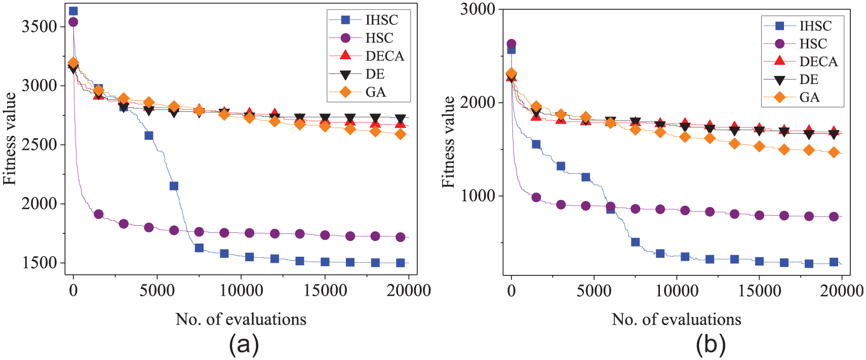
Convergence graph for case 3 in (a) WSN#1 and (b) WSN#2.

Figure 16.

Convergence graph for case 8 in (a) WSN#1 and (b) WSN#2.

Conclusion and future works

In this article, we propose an energy-efficient clustering and routing algorithm for WSNs, called IHSCR, which is based on HS algorithm. For dealing with the clustering problem, first, an objective function model, which has considered balancing the energy consumption of both gateways and regular nodes as well as considered routing, is established. Then, a new clustering approach, that is, IHSC algorithm, is developed based on four improvements made to the traditional HS algorithm: (1) an efficient discrete encoding scheme of a harmony (i.e. solution) for WSN clustering is proposed, which can contribute significantly to reducing the search space; (2) an efficient roulette wheel selection method is designed to choose a gateway for a regular node to join, which is employed by two steps (i.e. initialization of harmony and improvisation of a new harmony) and can contribute significantly to improving the convergence speed of IHSC algorithm; (3) the dynamically changed HMCR is designed for improvisation of a new harmony, which can make IHSC algorithm avoid prematurity and strengthen its global search ability in early iterations, and enhance its local search ability in late iterations; (4) a local search scheme is proposed to improve the best harmony within the HM in iterations, which can contribute significantly to improving the quality of the optimum found by IHSC algorithm. Besides, in the routing phase, the IHSBEER algorithm that we proposed previously is employed to calculate the forwarding paths for gateways, which can significantly balance the energy consumption of gateways. The proposed IHSCR is compared with HSCR, EELBCA, traditional GA- and DE-based clustering algorithms, and DECA over extensive WSNs cases. The experimental results clearly demonstrate that IHSCR has better performance than other clustering algorithms in terms of network lifetime, balance of the energy consumption of gateways and regular nodes, energy consumption, as well as convergence situation. In the future, we will implement IHSCR algorithm on a real WSNs to validate its effectiveness.