Sage Journals: Discover world-class research

Abstract

In this work, a two-stage architecture is used to analyze the information collected from several sensors. The first stage makes classifications from partial information of the entire target (i.e. from different points of view or from different kind of measures) using a simple artificial neural network as a classifier. In addition, the second stage aggregates all the estimations given by the ensemble in order to obtain the final classification. Four different ensembles methods are compared in the second stage: artificial neural network, plurality majority, basic weighted majority, and stochastic weighted majority. However, not only reliability is an important factor but also adaptation is critical when the ensemble is working in changing environments. Therefore, the artificial neural network and the plurality majority algorithm are compared against our two proposed adaptive algorithms. Unlike artificial neural network, majority methods do not require previous training. The effects of improving the first stage and how the system behaves when different perturbations are presented have been measured. Results have been obtained from two applications: a realistic one and another simpler one, with more training examples for a more accurate comparison. These results show that artificial neural network is the most accurate proposal, whereas the most innovative proposed stochastic weighted voting is the most adaptive one.

Keywords

Ensemble methods wireless sensor networks artificial neural networks voting algorithms classifier ensemble

Introduction

In the last years, the importance of wireless sensors networks (WSNs) has significantly increased as a consequence of the requirements of the Internet of Things (IoT). Systems tend to be more complex, using many sensors to sense a high number of variables and to “know” the environment around them in order to act properly. Consequently, these systems not only demand more communication and cooperation among their sensors but also need to be more intelligent and adaptive. In this work, some cooperative classifier ensemble methods are presented to combine estimations from sensors in order to obtain a more reliable solution. Besides, adaptation to changing environment is also tackled to determine how the system would be able to maintain a certain level of accuracy although external or internal conditions affect the system.

During the course of many years, several research activities have been focused on improving the behavior of intelligent systems using different artificial intelligent strategies. Particularly, decision making plays an important role under this topic since it can be used for different applications such as networks and energy management,^1–3 health care and medical decisions,^4,5 or autonomous transportation and road traffic^6–8 among others. Moreover, nowadays, systems tend to be increasingly more autonomous, and decisions have to be taken by themselves according to the environmental information. Furthermore, many of these systems have to be able to determine their behavior facing with changing environments or even to combine different responses provided by different sensors or agents in order to obtain a more accurate one. The application establishes the requirements; sometimes, reliability will be the most important aspect but performance, consumption, ease of deployment, or even adaptation are also other factors to be taken into account.

Pattern recognition is very related to decision making, and it is very extended in classification systems. One of the main characteristics of these systems is reliability, since classifiers need to be able to generate outputs with a high level of accuracy. Moreover, they allow us to predict the output of a specific event (usually once the system has been trained). There are many classification methods, such as artificial neural networks (ANNs), decision trees, K-nearest neighbors (KNNs), linear regression, or support vector machines (SVMs), which try to obtain a good classification of a training set in order to establish the best criteria for splitting and to label the data properly. In spite of the existing methods, several modifications of the original ones are being studied in order to improve the classification rates. Furthermore, the importance of this dependability requirement involves multiple efforts on developing new strategies to improve the system response.

Ensemble methods can improve the accuracy of a classification.^9–11 Usually, an ensemble is composed of two stages. Generally, it contains a primary set of learners, also called base learners, which are in charge of generating estimations for the second stage, which has to combine all of them. The most popular ensemble methods are bagging, boosting, stacked generalization, and ensembles of learners. All of them are based on creating several models using a training set. In case of bagging, models are built independently using different samples with replacement from the training set to obtain them. Once the models are created, they are ready to classify new samples. The same sample is applied as an input to every model, and the output is calculated as a combination of all single outputs (i.e. normally a mean or majority voting). Random forests are a special case of bagging. In this particular case, a set of decision trees are combined to obtain the final classification. Each decision tree–based model is built using a random selection of its attributes. Then, an input is applied to every model, and the final classification is given by the most popular class. In contrast to bagging, in boosting methods, a dependency among the models is defined. The most famous boosting method, called AdaBoost, was proposed by Freund and Schapire¹² in 1997. In this one, models are created sequentially, taking into account the behavior of the previous one. The samples tested in the previous model are weighted for the next one. In this way, the final classifier combines the votes of each individual classifier, where the vote of each one is weighted according to its accuracy. Although boosting methods are more accurate, the traditional ones usually risk overfitting the model.¹³ However, Schapire et al.¹⁴ demonstrated, through the margin theory, that AdaBoost has no indication of overfitting. Besides, random forests are often more robust to errors and even faster than traditional boosting. On the contrary, Wolpert defined the staked generalization¹⁵ as a two-level classifier in which the first one is an ensemble of classifiers whose outputs are used as input to the second level meta-classifier. Finally, an ensemble of learners combines different heterogeneous models. They use the training set to create different models using different algorithms (decision tree, KNN, linear regression, SVM, or ANN). All of these models are trained using the same training data set. Once the heterogeneous set of models is created, the same input is applied to every model, and all the single outputs are often combined using a mean operation. Usually, ensembles provide less error, so they are more accurate that bagging and booting, and they also decrease the overfitting and biases.

Kuncheva¹⁶ explains the importance of classifier ensembles and how the combination of several classifiers can improve the behavior of a classifier system. When different classifiers are combined, it is necessary to handle the contribution of each one to the finaldecision.^17–19 Therefore, an appropriated management of each classifier has to be previously defined. There are two main strategies to deal with the whole ensemble: (1) fusion and (2) selection. On one hand, a selection strategy is more focused on working with different specialized classifiers, which means that each one knows a specific part of the feature space and therefore is responsible for classifying the classes belonging to this part. On the other hand, classifier fusion approach is more focused on combining the contribution of every classifier in order to obtain another more accurate one.²⁰

In this work, we use the two-stage classifier ensemble architecture used in our previous work.²¹ It is composed of several individual classifiers which have to be combined in order to obtain the final result. The proposed architecture is shown in Figure 1.

Figure 1.

Proposed general scheme of the system.

The first stage provides some classifications obtained from partial information about the target, and then the second stage is in charge of combining all of them to obtain a final improved classification. Classifiers of the first stage have been implemented as ANNs (particularly as multi-layer perceptrons (MLPs)) trained with partial information about the target. The proposed methodologies of this work are focused on the second stage, where different methods will be employed to compare the efficiency and adaptability of each one. On one hand, another ANN will be implemented, whereas, on the other hand, different voting algorithms are also tested. This second-stage ANN needs to be trained, and it uses the estimations of the first stage as its inputs in order to generate the output of the ensemble. Related to the voting algorithms, three different methods are tested. The simplest one is plurality majority and the others are two proposals based on weighted majority, which are called basic weighted and stochastic weighted voting algorithms. In section Second stage: classifier ensemble, these algorithms are described in detail.

As mentioned before, bagging and booting methods use the same data set and split it using different techniques. In contrast, in this case, there are different data sets to be analyzed as a consequence of a multi-sensor scenario. This fact allows us to use the same algorithm (in this work, ANNs) for all the classifiers located in the first stage, because each one provides different results since they use different data sets. Although the proposal is not exactly an ensemble of learners in terms of heterogeneity, it can be considered as an ensemble method which deals with its own scenario. Three of the proposed algorithms are considered machine learning methods because they have some learning capabilities and take into account the previous system behavior. Therefore, in these cases, the proposal can be considered as a stacked generalization approach. Just in case of majority voting, this assumption is not certain, because it does not imply any kind of learning.

Moreover, not only accuracy has to be taken into account, adaptability is another characteristic to address. Therefore, this article introduces a comparison among adaptive and non-adaptive fusion algorithms in a two-stage classification scheme as an ensemble method mainly focused on the second stage. A classifier can be trained for a specific application and, consequently, it will carry out a great classification. However, if some changes affect the system, the classifier will provide worse results. Therefore, adaptability is a very important factor to consider a high level of reliability, even in classifier ensembles.^22,23 Hence, in this work, adaptive capabilities are also analyzed and compared depending on the algorithm used in the second stage.

In this article, we present improved results of the first stage from our previous work.²¹ Thus, the results of the second stage are also improved. This allow us to analyze the effect of the first-stage accuracy on the second stage. Besides, we present an additional application example which is more realistic and uses real data collected from sensors (in this case, low-cost radars).

This article is organized as follows. In section Example applications, the two example applications used to compare and test the algorithms are described. Then, in section First stage: preprocessing individual sensor data, the role of the first stage is discussed and the ANN used is described. Section Second stage: classifier ensemble describes the algorithms used in the second stage, which are then compared. Section Results of the detection with radars shows the results obtained for this application example. The comparison of the second-stage algorithms is shown in section Results of the multi-sensor MNIST application, where the perturbation effect is also analyzed. Discussion of the obtained results are shown in sections Results of the pedestrian and car detection and Results of the multi-sensor MNIST, where authors explain the advantages and disadvantages of each method. Finally, in section Conclusion and future lines, final conclusions are given and some future lines are also presented to show which could be the future steps to improve the system performance and the behavior of each algorithm. Figure 2 shows a graphic structure of the article.

Figure 2.

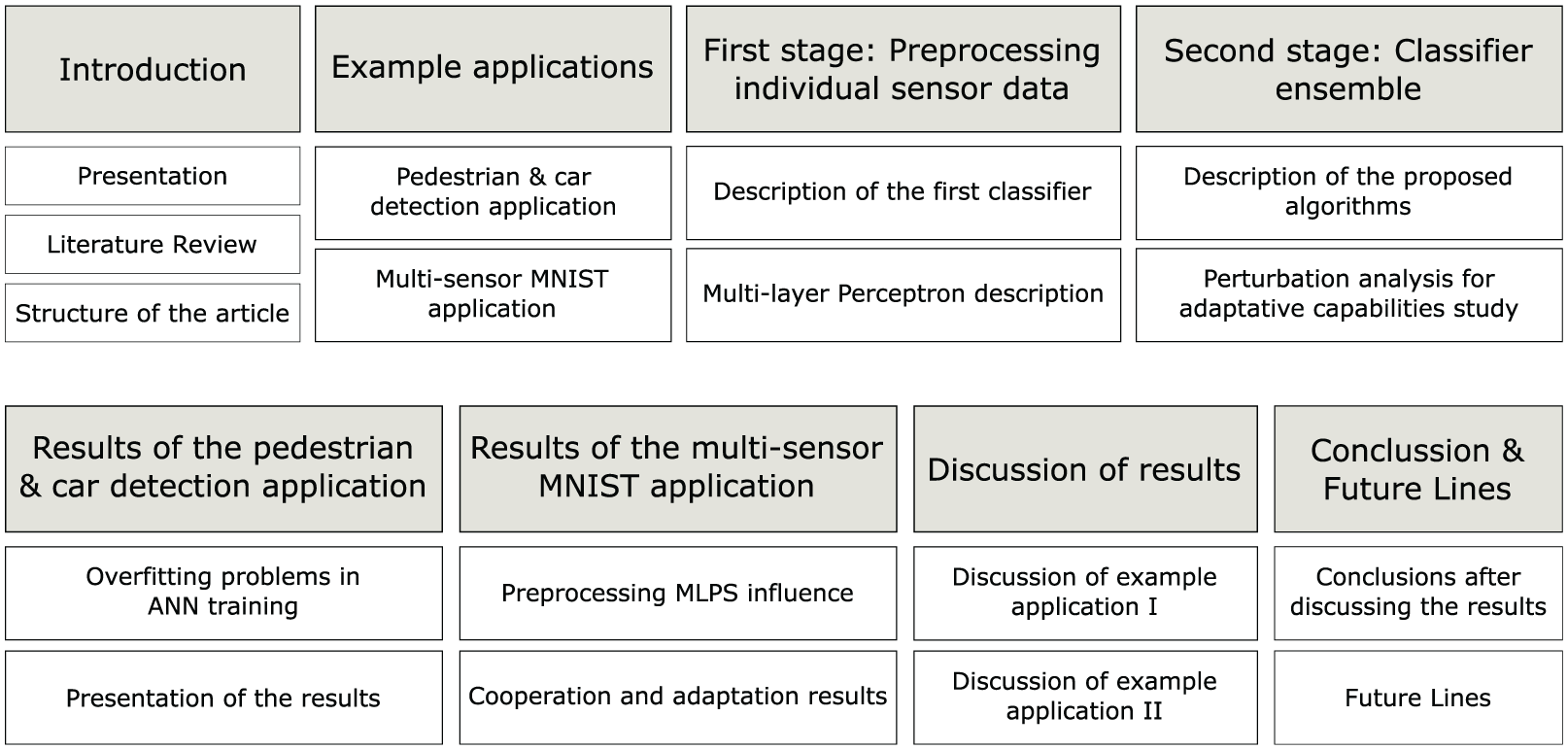
Structure of the article.

Example applications

As mentioned in the above section, this work makes a comparison among different algorithms for combining the outputs of a classifier ensemble. In order to test the proposed algorithms, different example applications have been analyzed. The first one consists of detecting and identifying cars and pedestrians using low-cost radars.²⁴ This is a realistic application where the position of the radar device is so critical, therefore collaboration among devices can be a solution to play down this problem. For this application, only a small set of samples is available since samples were taken in a complex environment. However, it is possible to analyze the behavior of each algorithm on the overall system testing different situations. In order to make a more detailed study, we have defined another example application. In this case, a huge data set is available, so a statistically relevant analysis of the algorithms can be performed since enough tagged examples are available. This second application is a modification of the well-known MNIST database²⁵ in order to adapt this database into our multi-sensor scenario. It was also the same application example used in our previous work,²¹ in which handwritten numbers had to be classified. Each device analyzes only a small part of the whole image, so the partial information is combined using the proposed algorithms. Although this application is not as realistic as expected, it is a good way to test the efficiency of the collaborative algorithms since we have enough samples to generalize the obtained results.

Pedestrian and car detection

Detecting cars, persons, animals, bikes, or another kinds of objects when they are moving is not a complicated task. The challenge resides in the classification to identify the kind of the moving object. Although if this is complicated enough in itself, this difficulty becomes higher when the sensor device is a low-cost radar and due to the fact that it has no complex and precise functions. In spite of the sensor having some limitations, the obtained results were acceptable.²⁴ However, the radar position was so critical. In order to minimize this influence, a combination of several radars working together improve the results.²⁶ Therefore, in this work, a comparison among different algorithms is analyzed to demonstrate the utility of the cooperation.

In this example application, three low-cost radars were used in order to detect and identify the moving object from different angles. A deployment of the system was carried out to obtain a data set with real tagged samples. The three radars were placed in the parking of our school (Figure 3) to take samples of moving objects. Tags were added manually. When each radar signal surpasses a threshold, the software tool saves 512 samples in a second and the time of the event. Then, the first 128 points of the fast Fourier transform (FFT) of the 512 points signals are introduced as inputs to the first-stage classifiers. In this case, instead of using a classification tree,^24,26 an ANN is used to provide the results of each radar device for this first stage.

Figure 3.

Deployment of a radar for measuring.

A critical aspect of this example application resides in the limitations of the environment. The place was not so friendly for taking the samples, since the environment was not very controlled. Many people were moving around and many times trees were moving, and the radars detected these movements and mixed them with moving people or vehicles. Therefore, taking the samples was not an easy task. These complications caused a lot of problems in obtaining enough samples to make an exhaustive analysis. In order to reduce this problem, different testing situations are studied, and another example application is also tested to be available as an statistically relevant analysis.

After this experiment, we achieved 128 valid tagged signals. Out of them, 92 belonged to pedestrians or group of pedestrians, 23 to cars, and 13 to bikes. As there were not enough examples to train and test, five sets of 52 pedestrian signals were taken randomly from the 92 ones, 13 cars were taken randomly from the 23 ones, and the 13 bikes have been used to train the ANNs. The five sets of the remaining 40 pedestrian signals, 10 cars, and 0 bikes were used as test sets.

Multi-sensor MNIST

In order to test the proposed algorithms with enough examples, the well-known MNIST database²⁵ has been chosen as an example application. To adapt this database into our multi-sensor scenario, the following modifications and methodologies have been done:

The 28 × 28 pixel images of the MNIST database have been divided into four 14 × 14 sub-images. This emulates four different sensors catching the same event, but each one has only partial information of the entire target. The image has been divided as follows: the top left corner of the image is the quadrant 1, quadrant 2 is the bottom left corner, quadrant 3 is the top right corner, and quadrant 4 is the bottom right one. Figure 4 shows an example.

Each 14 × 14 sub-image is processed by a two-layer MLP trained to classify its quadrant. Thus, four estimations are obtained, each one with different global accuracy and class accuracy, due to the fact that some quadrants will be more sensitive to certain numbers than others.

In order to test the adaptability of each algorithm, different types of perturbations have been added as noise on the image and as communication errors between stages.

Figure 4.

28 × 28 image of a handwritten 7 divided into four 14 × 14 images.

The MNIST database is composed of two sets, one for training stage and the other one to test the system. The Train set contains 60,000 examples, whereas the Test set only contains 10,000. The first-stage classifiers were trained using three different subsets of 10,000 examples taken randomly from the Train set. We call the rest of the examples, which belong to the Train set but were not used to train the first stage, as the Train^– sets. The Train^– sets were used to test the first stage and to train the second stage, whereas the Test set was used to test the first and second stages.

First stage: preprocessing individual sensor data

The main focus of this article is on the algorithms which aggregate data from all sensors. Therefore, data from sensors are preprocessed with the same algorithm for all the proposed experiments. A two-layer MLP with an output per class has been chosen to implement the first stage of the proposed scheme (see Figure 1). Nevertheless, whatever other classifier could be chosen for this propose.

Combination of the first-stage classifiers does not literally represent a combination of multiple solutions for the same target. The outputs of the first stage have been obtained by MLPs using different inputs. Each one uses only partial information or a different point of view of the global target. It means that there is a high likelihood to obtain different classifications for the same target at each MLP in the first stage since they have a huge dependency of received input (image of each quadrant or signal from different oriented radar). This implies that every partial solution is not well-balanced, because these results do not only depend on the internal functionality of the MLP but also on the external information partially received from the target (image of each quadrant or signal from different oriented radar).

MLP

The mathematical model of a neuron is shown in equations (1) and (2). This model performs a weighted sum of the inputs and then applies an activation function to the output. The activation function is usually a linear function or a sort of saturation function like sigmoid functions

$a_{i} = \sum_{j = 1}^{M} w_{ij} \cdot x_{j} + b_{i}$ (1)

$y_{i} = f (a_{i})$ (2)

with $i = 1, \dots, N$ , where $x_{j}$ is the input, $w_{ij}$ is the weight, $b_{i}$ is the bias, $f ()$ is the activation function, $y_{i}$ is the output, $M$ is the number of inputs, and $N$ is the number of neurons.

There are different families of ANNs. Each family has different connections, activation functions, and learning algorithms. In this work, MLPs have been implemented, which only allow feedforward connections and are trained with supervised learning. They have as many outputs as classes are needed to be classified. The output is trained to be 1 for the corresponding class and −1 for the other classes. However, the final output will be a set of values in the range [–1,1], representing the confidence for each class.

The learning algorithm most used for training MLPs is backpropagation. It is an approximate steepest descent algorithm which uses the mean square error (MSE) between the ANN output and the desired one as the fitness function, where $MSE = \frac{1}{n} \sum_{i = 1}^{n} (t_{i} - y_{i})^{2}$ , $t_{i}$ is the desired output (target vector) and $y_{i}$ is the current ANN output. The neuron weights are updated using the following formula

$Δ w_{ij} = - α \cdot \frac{\partial e^{2}}{\partial w_{ij}}$ (3)

where $e^{2}$ is the MSE and $α \in [0, 1]$ is a scalar coefficient called learning rate, which regulates how fast the ANN learns.

A variation of the standard backpropagation, variable learning rate,²⁷ has been used for training. The weight update is performed in batch mode. This means that weight increments for each training example are accumulated and then applied after all examples (in an epoch). The learning rate is also updated at the end of the epoch, following these rules:

If the new MSE is less than the previous one, the learning rate is increased $η$ times.

Else, if the new MSE is greater than the previous one, but no more than a certain percentage $ζ$ , the learning rate is maintained.

Else, the new MSE is greater than the previous one plus a certain percentage of it $(ζ)$ , learning rate is decreased $ρ$ times, and also weights from the previous epoch are recovered.

On the detection with radars application

Each radar signal is, first, applied a FFT and the first 128 points are taken (an example is shown in Figure 5); then it is classified by a 2-layer MLP with 128 inputs, four hidden neurons, and three output neurons. Each output neuron recognizes a class: pedestrian, car, or bike.

Figure 5.

Radar parameter extraction: example of person signal.

Due to the lack of tagged examples, the first-stage classification performance is very unstable (as shown in the section Results). Therefore, five sets of classifiers have been trained with different training sets generated as described in section Example applications.

As there is a big unbalance between classes on the achieved tagged examples, the impact on the MSE of each example is corrected proportionally to its class abundance. Particularly, the squared error of each example is multiplied by the total number of examples of the training set (78) and divided by the number of examples of its class on the training set (52 persons, 13 cars, and 13 bikes). Hence, on every epoch (as training is performed in batch mode), the influence of each class is balanced on the MSE, avoiding a tendency to classify every input as the most abundant class.

The parameters for the first-stage training are as follows: 1500 iterations, $ζ = 1.03$ , $η = 1.04$ , $ρ = 0.8$ , random initial weights and bias with uniform distribution in the range [–0.15,0.15], initial learning rate $10^{- 5}$ , and both layer’s activation functions are sigmoid functions between −1 and 1, and origin slope 1. In the learning algorithm, the derivatives of the sigmoid functions have been saturated with a minimum value of 0.1.

On the multi-sensor MNIST application

Each quadrant, into which the input images are divided, is classified by a two-layer MLP with 14 × 14 inputs, 40 hidden neurons, and 10 output neurons. Each output neuron recognizes a digit. This is a relatively small ANN compared to the state-of-the-art ones used to solve MNIST.²⁵ It has been done by design to fit the MLPs on embedded implementations, which have a limited number of resources. Consequently, these networks cannot be as effective as the MLPs implemented on powerful machines.

In order to perform a fair comparison of algorithms, three sets of classifiers have been trained with 10,000 different examples taken randomly from the Train set of the MNIST database.

The parameters for the first-stage training are as follows: 5000 iterations, $ζ = 1.03$ , $η = 1.04$ , $ρ = 0.8$ , random initial weights and bias with uniform distribution in the range [–0.15,0.15], initial learning rate $10^{- 5}$ , sigmoid activation function between −1 and 1 (origin slope 1) on the hidden layer, and saturated linear on −1 and +1 with slope 1 activation function on the output layer. To improve convergence of the learning algorithm, on the output layer, the activation function derivative has been replaced by the derivative of the sigmoid function and saturated with a minimum value of 0.1. Note that, in this case, the sigmoid derivative of the hidden layer has not been saturated. These parameters have been chosen after a non-exhaustive exploration guided by the authors’ knowledge.

It should be noticed that these parameters have been modified from the ones used in our previous experiments reported in Villaverde et al.²¹ Particularly, the iterations have been augmented from 1500 to 5000, the activation functions have been optimized, and minor changes are performed on the scripts that compute the training. It can model two types of classifiers: a weak one in the previous experiments²¹ and a strong one for the new experiments.

Second stage: classifier ensemble

The second stage of the proposed system (see Figure 1 for more details about the general scheme) is based on the main concept of classifier ensembles since it has to combine the outputs coming from different classifiers (MLP in this case). In particular, in this work, different fusion approaches have been implemented to consider the different outputs given by the first classification stage. Another MLP and three different cooperative algorithms are proposed: majority voting-based algorithm, basic weighted voting-based algorithm, and stochastic weighted voting-based algorithm.

Whereas the neural network requires a training stage before the normal operation to adjust the internal weights in order to provide the best results, the proposed cooperative algorithms do not require any kind of previous training. Besides, the weighted voting-based algorithms are always updating the contribution of each classifier to provide a result every time for each input and also adapting itself to the system’s changes (i.e. changes which affect the proper functionality of one or more classifiers). Unlike the proposed neural network and the majority voting algorithms, these ones take into account the past behavior of the system. In this way, they can decide which first-stage classifier is giving the best results as time goes forward and, consequently, give more importance to their contributions.

MLP-based algorithm on second stage

MLP has also been chosen as one of the algorithms to compare. It is more computationally intensive than the other proposed algorithms, but it can achieve better accuracy when it is trained properly.

On the detection with radars application

Seven MLPs of nine inputs (three from each radar), 12 hidden neurons, and three output neurons have been trained with the same training sets used to train the first-stage MLPs. So, the test sets can be used for testing the second stage too.

The training parameters for the second stage are as follows: 700 iterations, $ζ = 1.03$ , $η = 1.04$ , $ρ = 0.8$ , random initial weights and bias with uniform distribution in the range [–0.15,0.15], initial learning rate $10^{- 5}$ , and both layer’s activation functions are sigmoid functions between −1 and 1, and origin slope 1. In the learning algorithm, the derivatives of the sigmoid functions have been saturated with a minimum value of 0.1.

On the multi-sensor MNIST application

Five MLPs of 40 inputs (10 from each quadrant), 15 hidden neurons, and 10 outputs have been trained with each of the remaining signals which belong to the training set but were not used to train the first stage (Train^– sets). As there are three Train sets for the first stage, there are also three Train^– sets with 50,000 examples. Thus, 5 × 3 = 15 different MLPs for the second stage were trained (five MLPs per each one of the Train^– sets).

The training parameters are as follows: 4000 iterations, $ζ = 1.03$ , $η = 1.04$ , $ρ = 0.9$ , random initial weights and bias with uniform distribution on range [–0.15, 0.15], initial learning rate $10^{- 7}$ , sigmoid activation function between −1 and 1, and origin slope 1, on the hidden layer; and saturated linear on −1 and +1 (slope 1) activation function on the output layer. To improve convergence of the learning algorithm, on the output layer, the activation function derivative has been replaced by the derivative of the sigmoid function and saturated with a minimum value of 0.1. Note that, in this case, the sigmoid derivative of the hidden layer has not been saturated. These parameters have been chosen after a non-exhaustive exploration guided by the authors’ knowledge.

Majority voting-based algorithm

Majority voting can be classified as (1) unanimous, (2) simple, and (3) plurality. Unanimous implies that all classifiers agree. In case of simple majority, at least more than 50% of classifiers agree. Finally, in plurality voting, the solution is given by the most voted category. In this work, plurality voting will be addressed as the majority voting-based algorithm.

This is the simplest and the fastest proposed algorithm. However, it has an important disadvantage since this method produces ties, especially in the case of a an even number of classifiers. When a tie happens, the classifier does not provide a reliable solution. Therefore, it can generate a high level of uncertainty. Another disadvantage is produced when a first-stage classifier starts to provide wrong results (i.e. due to a change in the environment or to a internal failure). If the system does not realize that situation, the hit rate will get worse. This is due to the fact that the solution does not depend on the previous behavior, but this algorithm just analyzes the inputs and provides the result using only this information. Therefore, it is a non-adaptive methodology.

Basic weighted voting-based algorithm

Unlike the majority algorithm, the basic weighted voting weights each input to manage the contribution of each classifier. The functionality is very similar to the majority one. The solution is also the most voted category but, in this case, contributions are weighted. These classifiers which have demonstrated a higher reliability will have more influence over the final decision. The solution of every quadrant is compared to the final solution; if they match, this means that the classifier has contributed positively to the final decision, so its weight will be increased by adding a fixed value $δ_{+}$ . In contrast, if both results do not match, the weight of that classifier will be decreased by subtracting a fixed value $δ_{-}$ to reduce its influence for the future activity.²⁶ It means that the algorithm is continuously updating the weights and therefore it can adapt the system to external or internal changes, which affects the reliability of the classifiers. Figure 6 shows the pseudocode of this algorithm.

Figure 6.

Pseudocode for the basic weighted algorithm.

In this method, the fact that weights have to be increased or decreased using a predefined fixed value is the largest drawback. Although the increase can be a little more higher than the decrease (or vice versa) to avoid standstill, both parameters have to be predefined by the programmer. Moreover, initial weights $α_{0 i}$ ( $i = 1, . . ., N$ , where $N$ is the number of classifiers) are also important, and they have to be predefined too. All these values have a very important influence over the system evolution since the reliability of the system depends on how its weights are evolving. In this work, the predefined values have been $α_{0} = 0.5$ (all classifiers have the same initial weight), $δ_{+} = 0.5$ , and $δ_{-} = 0.025$ .

Stochastic weighted voting-based algorithm

This algorithm also weights the influence of each classifier. But unlike the basic weighting, in this case, weights are calculated using a stochastic method. Therefore, the programmer does not need to define how weights evolve, because they are updated based on the Monte Carlo method. Thus, this algorithm works similarly to a particle filter since it computes, every time, a large combination of weights (i.e. particles) in order to reach a good solution. In this work, 200 particles have been used. Initially, all particles are randomly distributed and cover all the available space. Then, as the algorithm proceeds, particles are continuously moving around the valid ones. If there is a change in the environment, particles will move to another area of the space in order to accomplish the new requirements and maintain more or less the same level of accuracy. The final weights are not given by a specific particle, but they are calculated according the distribution of all particles (particularly, by the geometric center of all particles).

The available space for particle location is limited, and the coordinates of each one can vary only between 0 and 1. Although, at the first time, particles are randomly distributed in all the space, for next launches, they will be only distributed around the valid ones. In this way, the convergence of the particles is searched to find the best space of particles according to the solutions given by the classifiers. The final weights will be calculated as the geometric center of each coordinate of every particle, where each coordinate represents the weight of each classifier. Every particle is evaluated to determine which ones are valid giving a final solution. This result is compared with the result calculated using the geometric center. If both results match, then that particle is considered a valid combination, otherwise it will be rejected. However, not all the particles are equally valid. Some of them will have a strong contribution and consequently, the final weight combination will be closer to them. In order to find these particles, a deeper analysis of them is required.

Once the weights provided by a particle are applied to calculate the result for that particle, it is possible to know which is the dispersion around the different categories. It means that when the weights given by a particle are applied, the result will be determined by the category which has the highest contribution. However, other categories could also have some contribution. As these contributions are more similar, the result is less reliable since the system cannot distinguish a single solution well. In contrast, if one category obtains much more contributions than the others, it means that the result presents more confidence $(γ)$ . Consequently, particles which provide a more distributed result among the categories will have less particles around themselves in the next launch. On the contrary, if the resulting category provided by a specific particle has a higher contribution regarding the others categories, then that particle will have more of them around itself for the next launch. Figure 7 shows an example for calculating the final result of two specific particles, $A$ and $B$ , assuming that both are valid particles (i.e. their final results match the result calculated using the geometric center). In this example, quadrants 1 and 3 classify the input as category 8, and quadrants 2 and 4 identify the category 3. Taking into account the results given by the quadrants, when the particle $A = [0.81, 0.62, 0.54, 0.35]$ is evaluated, its result is category 8, since the sum of contributions of quadrants 1 and 3 is higher that the sum of contributions for the others quadrants. In contrast, although particle $B = [0.73, 0.38, 0.89, 0.46]$ provides also the same category, its confidence is higher since the difference between category 8 and 3 is higher in this case, and therefore, there will be more particles around particle $B$ than around particle $A$ in the next launch. The pseudocode of this algorithm is shown in Figure 8.

Figure 7.

Example of the final result calculation for two valid particles.

Figure 8.

Pseudocode for the stochastic weighted algorithm: computer version.

In conclusion, this algorithm is also adaptive like the basic weighted voting-based algorithm, but, unlike the previous one, this takes its own decision about evolution of weights by itself. There is no need to predefine a fixed value to reward or penalize the first-stage classifiers. The algorithm decides how to do that by moving the particles over the available space according to the behavior of each one. Therefore rewards and penalties will be different every time.

Perturbations

Different perturbations have been added to the Test set of the multi-sensor MNIST application in order to check the adaptability of the proposed algorithms. These perturbations can affect the inputs or the link between the first and the second stage. Sensor malfunctions or image corruptions can cause some failures in the input of the first stage. On the contrary, external noise can affect the link between the first and the second stage (especially if both stages are placed in different locations). Consequently, the input of the second stage may be corrupted or even the connection may be lost. In this work, corruption in both first and third quadrants has been studied to analyze the influence of each one over the global system, representing failure not only of one of the best quadrants but also of one of the worst ones (see Table 2 for quadrant performances).

Initially, the image noise associated to different quadrants was added to simulate the first case (image noise). The first quadrant was corrupted with additive Gaussian noise (adding a normal distribution noise with mean 0 and standard deviation of 64), which is the most frequently used. Then, the analysis was repeated applying the same type of noise on the third quadrant instead of the first one. On the contrary, some noise was also added over the output of the first stage, therefore data received in the second one was partially corrupted. Different situations were analyzed. Gaussian noise with a standard deviation of 1 and 0.5 was applied to study two different cases with different noise levels. Besides, in order to simulate a disconnection, the input of the second stage was replaced by the less worse case possible. For the ANN, it is all outputs fixed to −1, which represent “no-idea,” and a random assignment for the rest of algorithms which have to vote an hypothesis. Like the previous case, the first and the third quadrants were being corrupted separately.

Therefore, four different perturbations have been analyzed. One of them as a image noise and the others as noise in the link between the first and the second stage. For each case, experiments were done when the failures were associated not only to the first quadrant but also to the third one.

Results of the pedestrian and car detection application

The lack of tagged examples causes overfitting problems in the ANN training. Figure 9 shows the evolution of the MSE of the train and test sets during a training of a first-stage MLP. The overfitting problem is when the MSE of the training set improves by learning each training example with precision, whereas the ANN loses generalization and the MSE of the test set decreases. It appears when there are more learning parameters (i.e. weight and bias) than training examples, after some training epochs. As more learning parameters than training examples are present, the sooner (i.e. at earlier epoch) appears the problem. In this case, as there are few training examples, the size and/or the training epochs are limited, and hence the performance of the MLPs. Besides, it also causes the training of the first stage MLPs to be very unstable (getting very different results on each experiment). Therefore, we have chosen five different situations of the first-stage MLPs as examples of how the algorithms may work instead of averaging them.

Figure 9.

Example of overfitting on the training of first-stage MLP.

Table 1 shows the results on the test sets of the detection with the low-cost radars. As shown in the firsts three rows of Table 1, there is not a clear tendency for every test, therefore each test is analyzed as a particular test to show how it affects the overall system (see section Conclusions for example application I).

Table 1.

Results in % of the detection with low-cost radars.

	Test 1			Test 2			Test 3			Test 4			Test 5
	Hits	Ties	Miss	Hits	Ties	Miss	Hits	Ties	Miss	Hits	Ties	Miss	Hits	Ties	Miss
Radar 1	82	0	18	76	0	24	86	0	14	78	0	22	84	0	16
Radar 2	78	0	22	84	0	16	80	0	20	84	0	16	82	0	18
Radar 3	94	0	6	86	0	14	86	0	14	84	0	16	88	0	12
ANN	97	0	3	92	0	8	90	0	10	88	0	12	87	0	13
Majority	94	0	6	90	4	6	94	0	6	90	4	6	92	6	2
Basic weighted	94	0	6	90	4	6	94	0	6	90	4	6	92	6	2
Stochastic weighted	94	0	6	90	0	10	94	0	6	92	0	8	96	0	4

Results of the multi-sensor MNIST application

Although, in this work, the first stage is not one of the main issues to be dealt with, it plays an important role in understanding the results of the second stage. Therefore, first, an analysis of the MLPs of the first stage is done in order to know the starting point. Then, results for the ensemble classifier are shown to compare the four cooperative algorithms explained above.

Besides accuracy, the other important issue dealt in this work is the adaptability. Adaptive capabilities allow us to maintain the system with a similar level of accuracy although external or internal conditions affect the system or their components. Therefore, in order to demonstrate these capabilities, some perturbations were introduced to analyze the system response.

Preprocessing MLPs

Due to the fact that images have been divided into four quadrants, the accuracy of each one is different. In order to know the behavior of each quadrant, different data subsets of the MNIST database were tested.

Table 2 shows the accuracy for each quadrant on the new experiments, whereas Table 3 shows the accuracy on our previous experiments. In order to avoid outliers, three experiments were developed for each case. Therefore, values shown in these tables were obtained as a median after the three experiments were carried out under the same conditions but using different subsets of samples. Besides, these tables also show not only the global accuracy but also the values obtained for each category. In this way, it is possible to discover where the categories are more difficult to classify (which turns to be the number “5”).

Table 2.

Accuracy in % of the preprocessing classification from the new experiments.

	Quadrant	0	1	2	3	4	5	6	7	8	9	Global
Train^–	1	66	94	72	81	75	37	74	84	66	73	73
	2	94	93	80	70	71	52	90	91	80	76	80
	3	91	95	65	72	88	90	92	85	63	74	82
	4	91	94	85	57	68	43	80	78	67	70	74
Test	1	69	95	74	84	78	36	76	82	68	72	74
	2	94	94	80	74	71	49	88	92	80	76	80
	3	92	97	67	76	88	91	91	83	59	77	82
	4	93	94	85	61	71	43	80	77	64	74	75

For each class, the median of the three experiments (to avoid outliers) and for the global accuracy, the mean (of the three experiments) are given.

Table 3.

Accuracy in % of the preprocessing classification from the previous experiments.²¹

	Quadrant	0	1	2	3	4	5	6	7	8	9	Global
Train^–	1	61	91	65	71	63	12	57	77	56	59	62
	2	91	89	66	63	68	15	84	75	67	46	67
	3	87	93	48	44	61	64	82	74	43	60	66
	4	89	92	69	51	57	5	74	73	53	59	63
Test	1	65	93	67	73	65	11	62	75	58	60	64
	2	92	90	64	65	68	15	82	75	66	45	67
	3	87	93	50	49	63	61	82	72	40	62	66
	4	93	91	72	55	58	6	76	73	52	64	65

For each class, the median of the three experiments (to avoid outliers) and for the global accuracy, the mean (of the three experiments) are given.

A big improvement can be noticed from the previous experiments to the newly optimized ones. We will take advantage of this fact to compare the second-stage algorithms against this two different situations. On one hand, our previous experiments represent a situation with a low-accurate first stage.²¹ Let us call this first stage as weak classifiers. On the other hand, the new experiments have a first stage with higher accuracy. Hence, let us call them as strong classifiers.

Comparing the global accuracy of the Test results from the new experiments against the old ones using equation (5) (see next subsection), we get 29.20% on quadrant 1, 40.35% on quadrant 2, 46.94% on quadrant 3, and 28.47% on quadrant 4.

Cooperative algorithms and adaptive capabilities

Once the accuracy of each quadrant is known, data fusion is analyzed. It implies to study how each algorithm works in terms of accuracy and adaptation. As mentioned before, in this work, four algorithms have been presented.

The system evolution when a change affects it denotes the system susceptibility and, consequently, how it can maintain a certain level of accuracy when a perturbation appears. Trained systems tend to be more unstable when facing environmental changes. In contrast, they used to be more accurate since the training stage provides them with some knowledge in advance. As mentioned in subsection Perturbations, different perturbations were applied in different parts of the system independently. Table 4 shows (1) the accuracy for each algorithm without any kind of noise and (2) how this accuracy is affected when these perturbations are applied. Table 5 shows the accuracy of our previous experiments for the same cases.

Table 4.

Accuracy and adaptability of the proposed algorithms for the second stage when the first stage has high accuracy (new experiments).

	ANN		Majority			Basic weighted			Stochastic weighted
	Hits	Miss	Hits	Ties	Miss	Hits	Ties	Miss	Hits	Miss
No perturbation	96.21	3.79	84.14	11.68	4.18	87.36	5.62	7.02	89.22	10.78
Im. Q1 Gaussian 64	95.46	4.54	81.48	13.75	4.77	86.25	5.78	7.97	88.14	11.86
Im. Q3 Gaussian 64	95.54	4.46	81.88	13.43	4.69	86.26	6.07	7.67	88.23	11.77
Link Q1 discon.	94.01	5.99	70.91	24.18	4.91	83.64	8.52	7.84	86.08	13.92
Link Q3 discon.	92.60	7.40	65.81	28.41	5.79	82.10	10.67	7.23	85.07	14.93
Link Q1 Gaussian 0.5	94.95	5.05	81.48	14.17	4.35	86.31	5.89	7.80	88.22	11.78
Link Q3 Gaussian 0.5	95.20	4.80	82.06	13.71	4.23	86.53	6.16	7.31	88.41	11.59
Link Q1 Gaussian 1	90.65	9.35	76.55	18.95	4.50	85.23	5.79	8.97	87.05	12.95
Link Q3 Gaussian 1	91.38	8.62	75.22	19.99	4.79	84.51	7.04	8.45	86.74	13.26

Table 5.

Accuracy and adaptability of the proposed algorithms for the second stage when the first stage has low accuracy (old experiments).²¹

	ANN		Majority			Basic weighted			Stochastic weighted
	Hits	Miss	Hits	Ties	Miss	Hits	Ties	Miss	Hits	Miss
No perturbation	90.72	9.28	68.46	23.17	8.37	74.87	10.79	14.34	77.57	22.43
Im. Q1 Gaussian 64	88.01	11.99	61.05	29.08	9.87	72.25	11.21	16.54	75.10	24.90
Im. Q3 Gaussian 64	89.39	10.61	65.00	25.69	9.31	73.85	11.13	15.02	76.52	23.48
Link Q1 discon.	82.92	17.08	52.49	38.46	9.05	68.60	18.39	13.01	73.32	26.68
Link Q3 discon.	82.44	17.56	51.97	39.16	8.87	69.58	18.10	12.32	74.03	25.97
Link Q1 Gaussian 0.5	86.07	13.93	63.11	28.05	8.84	72.90	11.75	15.35	76.02	23.98
Link Q3 Gaussian 0.5	85.47	14.53	62.54	28.36	9.10	73.05	11.71	15.24	75.88	24.12
Link Q1 Gaussian 1	75.36	24.64	57.72	33.32	8.96	71.73	11.67	16.61	74.64	25.36
Link Q3 Gaussian 1	72.42	27.58	57.10	33.51	9.39	72.17	11.69	16.14	74.63	25.37

Figures 10 and 11 show the influence of noise over the non-perturbation case for each algorithms of both new and previous data, respectively. They represent the difference between the hit rates without any perturbation and the hit rates when different perturbations were applied using, in the first stage, the weak classifier (our previous experiments) and the strong classifier (our new experiments), respectively (applying equation 4). The values of these hit rates are obtained from Tables 3 and 2. These two figures highlight the influence of the accuracy of the first stage over the global result for each algorithm. The ANN shows the most important variation. When a weak classifier is used in the first stage, the ANN of the second stage is more sensitive to noise, as our previous results demonstrate. However, for the new experiments, the ANNs of the first stage are more accurate, therefore the ANN of the second stage suffers less variation when the perturbations are applied. Although these effects are also presented for the other algorithms, the influence is not as significant as the ANN case

$error = Hit s_{original} - Hit s_{perturb}$ (4)

Figure 10.

Comparison graph for previous experiments (hits analysis).

Figure 11.

Comparison graph for new experiments (hits analysis).

In order to know how good the weighted algorithms are, adaptive capabilities have been analyzed taking into account the percentage of failures (miss + ties) of every algorithm when the perturbations are applied. These percentages are shown in Tables 6 and 7 and have been obtained using the formula

$θ = \frac{(Miss + Ties - (Miss' + Ties')) * 100}{Miss + Ties}$ (5)

where $Miss + Ties$ is the number of failures when no perturbation is applied and $Miss' + Ties'$ is the number of failures when the perturbation is presented.

Table 6.

Percentage of failure increase of the perturbations for the new experiments.

	ANN	Majority	Basic weighted	Stochastic weighted
Im. Q1 Gaussian 64	19.75	16.77	8.78	10.02
Im. Q3 Gaussian 64	17.73	14.25	8.70	9.18
Link Q1 discon.	58.23	83.42	29.43	29.13
Link Q3 discon.	95.39	115.64	41.61	38.50
Link Q1 Gaussian 0.5	33.37	16.77	8.31	9.28
Link Q3 Gaussian 0.5	26.61	13.11	6.57	7.51
Link Q1 Gaussian 1	146.73	47.86	16.77	20.13
Link Q3 Gaussian 1	127.47	56.24	22.55	23.01

Table 7.

Percentage of failure increase of the perturbations for the old experiments.

	ANN	Majority	Basic weighted	Stochastic weighted
Im. Q1 Gaussian 64	29.20	23.49	10.43	11.01
Im. Q3 Gaussian 64	14.33	10.97	4.06	4.68
Link Q1 discon.	84.05	50.63	24.95	18.95
Link Q3 discon.	89.22	52.28	21.05	15.78
Link Q1 Gaussian 0.5	50.11	16.96	7.84	6.91
Link Q3 Gaussian 0.5	56.57	18.77	7.24	7.53
Link Q1 Gaussian 1	165.52	34.05	12.53	13.06
Link Q3 Gaussian 1	197.20	36.02	10.74	13.11

Figures 10 and 11 also provide this information; however, we use equation (5) as an additional analysis because when the hit rate is closer to 100%, it becomes more difficult to improve it. Thus, using equation (5), for a low failure rate, a small improvement becomes as relevant as a big improvement for a high failure rate.

In order to obtain the ANN results, the second stage MLP was trained five times per each one of the three Train^– sets (defined in subsection MLP-based algorithm on second stage). The other algorithms do not need to be trained. Then, each perturbation kind has been generated three times per each one of the three training subsets. Finally, results has been averaged. Therefore, results in Tables 4 and 5 are the mean of (1) 15 experiments for the “No perturbation” case of ANN algorithm, (2) 3 experiments for the “No perturbation” case for the other algorithms, (3) 45 experiments for each perturbation on ANN algorithm, and (4) 9 experiments for each perturbation on the other algorithms.

A remarkable issue of these results is that two of the proposed algorithms show some kind of uncertainty due to the appearance of ties. When an algorithm generates not only hits and misses but also ties, it means that it is not robust enough. Consequently, ties introduce an important level of uncertainty in the system since it is not possible to provide a specific solution. These ties would be hits or misses, which depends on the number of ties and on the number of involved categories. It could be an important factor to take into account according to the application requirements.

In order to analyze the influence of the first stage into the second stage, Table 8 shows the improvement of the failure rates (ties + miss) when comparing the new experiments (strong classifiers) against the old ones (weak classifiers). These percentages have been calculated using equation 5, but in this case, we use $Miss + Ties$ as failures of the weak classifiers and $Miss' + Ties'$ as failures of the strong classifiers.

Table 8.

Percentage of failure improvement of the new experiments with respect to the previous ones, calculated using equation (5).

	ANN	Majority	Basic weighted	Stochastic weighted
No perturbation	59.17	49.71	49.70	51.94
Im. Q1 Gaussian 64	62.16	52.45	50.45	52.37
Im. Q3 Gaussian 64	57.96	48.23	47.46	49.87
Link Q1 discon.	64.90	38.77	47.90	47.83
Link Q3 discon.	57.84	28.79	41.16	42.51
Link Q1 Gaussian 0.5	63.73	49.80	49.48	50.88
Link Q3 Gaussian 0.5	66.99	52.11	50.02	51.95
Link Q1 Gaussian 1	62.06	44.54	47.81	48.94
Link Q3 Gaussian 1	68.75	42.24	44.34	47.73

Discussion of results

Discussion of example application I: pedestrian and car detection

As we have mentioned before, the samples obtained for the pedestrian and car detection application are limited. Therefore, the results of this application example are not statistically relevant and consist of analyzing different successful test cases.

In general, the second stage is able to obtain better results than each radar individually. It means that the ensemble improves the success rate of the individual classifiers. However, in one case, the ensemble cannot exceed the best individual rate. This effect happened in the Test 1 (in Table 1) where most of the algorithms are not able to improve the best individual radar result (from Radar 3). Only the ANN improves a 3% of that value. On the contrary, in Test 5, ANN shows worse results than the best individual radar rate. However, for this test, the best improvement is given by stochastic weighted voting-based algorithm, which surpasses 8% of the best individual result. In all the other tests, all the algorithms of the second stage are able to exceed the best individual rate, therefore the classifier ensemble can be a good alternative to improve the system behavior.

In general, ANNs present good results when there are enough samples to train. However, there are some tests in which the ANN does not provide better results than the other algorithms. This is due to the fact that the number of samples in this application are very limited and, in consequence, the ANNs are not well-trained. This means that the other algorithms can be preferred than ANNs when the application cannot provide a huge number of tagged samples. Even majority gives better results than ANN for tests number 3, 4, and 5. However, in these cases, the best alternative is the stochastic weighted voting-based algorithm, since it provides the highest hit rate (due to its adaptive capabilities) and also reduces the system uncertainty because it does not present any tie.

It is important to notice that even if these results are not statistically relevant, we have found examples in which the classifier ensemble improves the best individual classifier (those improvements are between 3% and 8% depending on the cases), proving so, the usefulness of a classifier ensemble with the tested algorithms in a real application.

Discussion of example application II: multi-sensor MNIST

All the results provided in this article have been obtained through MATLAB simulations, although the final implementations are intended to be executed in embedded platforms (micro-controllers, digital signal processors (DSPs), or field-programmable gate arrays (FPGAs)). The estimated number of operations needed to generate a decision from the four first-stage outputs are as follows: 800 for the ANN (already trained), 18 for the majority, 26 for the basic weighted, and $~ 2800$ for the stochastic weighted. These are rough estimations of basic operations that may have different complexities (e.g. increments, additions, multiplications, comparisons, divisions, etc.). Depending on the implementation platform, different levels of parallelism can be exploited, and each operation has a different execution time.

First of all, it is important to highlight that some results were obtained previously²¹ for this application. The differences between our first results and the new ones are basically found in the first stage. In this work, the ANNs of the first stage (preprocessing MLPs) have been improved and therefore the results for the second stage have also changed. As Tables 2 and 3 show, the accuracy of the new ANNs is better than the previous one for every quadrant for both Train^– and Test sample sets. It implies more confidence data to be dealt in the second stage and, consequently, high accuracy is obtained in the new experiments. Improving the first stage, the ANN for the second stage is able to suffer less deterioration (see Figures 10 and 11). Results of the preprocessing MLPs on the new experiments show that the accuracy varies a 9% among all quadrants since the best one has a hit rate of 82%, whereas the worst one is around 73% (see Table 2). According to these results, quadrants 2 and 3 are the best ones, which coincides with the best ones in our previous experiments.²¹ Besides, there are some categories more complicated to classify than others. The most significant case is obtained for category 5, since the lowest values belong to that category. It means that when the image represents the number five, all quadrants, except the third one, have some difficulties to classify it correctly, which again coincides with the previous experiments. This is one of the main reasons to choose quadrant 3, instead of quadrant 2, to analyze the system response when some perturbations are applied in one of the best quadrants. In any case, the shown values indicate that all quadrants are not extremely accurate since the hit rate does not exceed the 82% in any case. It is due to the fact that dividing the image into four quadrants, the information of each one is reduced and, consequently, the difficulty to classify properly increases. This analysis concludes that all conclusions of this work can be extensible to any other application in which sensors are not so much accurate and the combination of multiple of their partial solutions can improve the system performance. In these terms, data fusion improves the accuracy of the system, regardless if the first stage is improved, as Tables 4 and 5 show, even when perturbations affects the system (except in some cases where majority voting algorithm is applied). These results demonstrate that, in general, the analyzed algorithms for cooperation are able to improve the individual hit rates. However, each one has some advantages and disadvantages and presents more or less improvements.

The first stage classifier has a great influence on the accuracy of the whole system. Using a strong classifier in the first stage implies better general results because when the accuracy of the first stage improves, the accuracy of the second stage also improves. As we have defined before, Table 8 shows the percentage of failure improvement comparing the previous experiments (which use a weak classifier) with the new experiments (which use a strong classifier). According to those values, when there is no perturbation in the system, the ANN can improve a 59.17%, whereas the three majority-based algorithms can improve around 50%. The stochastic weighted is voted the best of the three since it has 51.94% of failure improvement. This demonstrates that the ANN of the second stage provides the highest improvement compared to the other algorithms since it has been trained with more new reliable samples. Therefore, when an algorithm requires a training stage before the commissioning, it can present best result than other non-trained algorithms; however, the second ones are able to work directly, also giving good results. Therefore, depending on the application requirements or limitation, we can choose one algorithm or the other one.

On one hand, regarding to the system hit rate, the ANN gives the best results. Its worst hit rate was around 73% in case of the previous experiments (see “Link Q1 Gaussian 1” and “Link Q1 Gaussian 1” in Table 5) which was improved in the new experiments reaching around 91% for the same kind of noise (see “Link Q1 Gaussian 1” and “Link Q3 Gaussian 1” in Table 4). In contrast, plurality majority presents the worst hit rates in any case; in some cases, this algorithm can only achieves a 55% or 60% of hits rates, especially when the first stage is not good enough (see Table 4). However, when a weighted algorithm is used, those values increase a lot compared with the plurality majority. In particular, for the new experiments, stochastic weighted voting can almost reach 90% of hits when no perturbation is applied (see Table 4), which only differs by 6% when compared with the ANN. Moreover, although the ANN continues getting better hit rates when perturbations are applied, the stochastic weighted voting does not have significant variations in presence of those perturbations. It means that it is more stable than ANNs for changing environments.

Therefore, regarding the system adaptation, we can conclude that the ANN is highly sensitive to any perturbations, especially when the accuracy of the first stage is lower. When a weak classifier (previous experiments)²¹ is used in the first stage instead of an strong one (new experiments), the ANN of the second stage suffers a significant deterioration. The error of the ANN when Gaussian noise with standard deviation 1 is applied can reach more than 15%–18% with respect to the non perturbed situation when a weak classifier is used in the first stage (see Figure 10). However, these values can be minimized under 6% when an strong classifier is used (see Figure 11). With respect to other algorithms, they can also minimize the error except when quadrant 3 suffers a link disconnection between both stages. In this case, the ANN is the only algorithm that can minimize the error. In this situation, the ANN algorithm has much more information than the other algorithms because when a disconnection is detected, the ANN can force all the input values for that quadrant to “ $- 1$ ,” which implies “no-idea” and, consequently, the algorithm can combine all inputs taking into account that the disconnected quadrant is not sure about its own results. However, the other algorithms have no available information, and they have to deal with a random value which will probably be wrong.

According to Table 8, the improvement that the ANN can reach is between 57.84% and 68.75%, whereas the stochastic weighted algorithm can only improve between 42.51% and 52.77%. This is a consequence of using a weak or strong classifier in the first stage, because the ANN (which is a trained method) is the most sensitive algorithm to any change in the first stage. As we have mentioned before, although the ANN has better hit rates in presence of perturbations than the other algorithms, its deterioration when those perturbations are presented shows a steep fall since the percentage of failures grows significantly, as Tables 6 and 7 show. In fact, in presence of some link noise (i.e. link Gaussian noise with standard deviation 1), the increment of the failure rate is even more than three times than the increment of the failure rate without perturbation. For example, when that noise is applied to quadrant 1, the ANN failure rate increases 146.73% in case of the new experiments and a 165.52% in case of the previous experiments (see Tables 6 and 7). In contrast, the failure rate of weighted algorithms does not exceed 38.50% for stochastic weighting and 41.61% for basic weighting for the worst case, as Table 6 shows. That is because ANNs are usually trained for general cases (i.e. without so many perturbations). Thus, when an unexpected perturbation appears, re-training will be necessary to adapt to the system, which involves getting new tagged examples of the perturbations. Furthermore, re-training may be impossible for some kind of applications or for sporadic perturbations. Therefore, in general, weighted algorithms are better in terms of adaptation than the ANN.

The ANN is also computationally very intensive. In this sense, the best algorithm may be the plurality majority, which is the simplest among all. It does improve the best first stage hit rate (except in the rare scenario of the Test 1 of the detection application with radars, in which it at least equals this value) when there are no perturbations. However, it does not obtain a significant improvement, and its accuracy decreases significantly with perturbations, specially for disconnections and intense noise on the link (Gaussian noise with standard deviation 1). The second computational effective algorithm is the basic weighted, which also provides balanced properties regarding accuracy and adaptability.

Conclusion and future lines

Conclusion

This article has compared four different algorithms for getting the final classification in a two-staged classifier ensemble. These algorithms have been applied to two example applications. Through the first application, the applicability of the classifier ensemble has been proven, testing the four proposed algorithms in a real application. On the contrary, through the second application, the proposed algorithms have been tested against different perturbations in order to measure their adaptability to environmental changes. Moreover, the effect of improving the accuracy of the first-stage classifiers has been measured.

After the discussion of the results, it can be concluded that

ANNs show the best accuracy among all the algorithms tested. However, they need to be trained with enough labeled examples, which for some applications will be unavailable or difficult to get. They have high computational intensity, and they are less adaptable than the weighted algorithms.

Majority shows the worst results in accuracy and adaptability (actually, it is not an adaptive method) and produces a lot of ties. It has been compared to show a reference of the minimum achievable improvement of an ensemble with the simplest algorithm. Nevertheless, it does improve the first-stage accuracy while providing the minimum computational intensity, which may be required for some applications.

Basic weighted shows intermediate and balanced results for accuracy, adaptability, and computation intensity. However, its main drawback is the ties generation, which produce a high level of uncertainty. This situation is not suitable for most of the applications since the unknown results can interfere with the system reliability.

Stochastic weighted shows the second best accuracy and the best adaptability. Although the hit rates do not reach the ANN results, they do not require any training before commissioning. Moreover, it shows a high level of adaptation because perturbations do not affect a lot due to its adaptive capabilities. Its main drawback is its high computational intensity. However, authors expect that by improving the particle selection stage, it will be possible to increase the hit rates and even reduce the computational efforts.

Future lines

Future lines will address the improvement of the stochastic weighted algorithm since it demonstrates low uncertainty due to the fact that it does not produce any tie, it also presents a high level of adaptation, and it does not required any type of training. Although it shows these great advantages, the main problem is its hit rate. Therefore, future research efforts could tackle this issue by changing the mode of particles selection or even the way to evolve them. Nevertheless, as Table 4 shows, for some specific cases under certain perturbations, the stochastic weighted algorithm can already exceed the ANN hit rate (i.e. when quadrant 3 is perturbed with Gaussian noise with standard deviation of 1 over the input of the second stage for a low accuracy first stage, old experiments). Therefore, if the stochastic weighted algorithm is improved enough, it will be a better option than ANNs for sensors data fusion in critical applications with changing environments.

Footnotes

The authors would like to thank José M Pardo and Marta Álvarez for their help.

Handling Editor: Hiram Ponce

Declaration of conflicting interests

The author(s) declared no potential conflicts of interest with respect to the research,authorship,and/or publication of this article.

Funding

The author(s) disclosed receipt of the following financial support for the research,authorship,and/or publication of this article: The work was partially supported by the Spanish Ministry of Education,Culture and Sport (FPU grant program FPU13/04424) and by the Universidad Politécnica de Madrid (Programa propio RR01/2015).

ORCID iD

David Aledo

References

Shahnia

Bourbour

Ghosh

Coupling neighboring microgrids for overload management based on dynamic multicriteria decision-making. IEEE T Smart Grid 2017; 8(2): 969–983.

Lee

Sriram

Kim

et al . Vertical handoff decision algorithms for providing optimized performance in heterogeneous wireless networks. IEEE T Veh Technol 2009; 58(2): 865–881.

Niyato

Hossain

Dynamics of network selection in heterogeneous wireless networks: an evolutionary game approach. IEEE T Veh Technol 2009; 58(4): 2008–2017.

Yang

Jin

Mummert

et al . A boosting framework for visuality-preserving distance metric learning and its application to medical image retrieval. IEEE T Pattern Anal Mach Intell 2010; 32(1): 30–44.

Rahulamathavan

Veluru

Phan

RCW

et al . Privacy-preserving clinical decision support system using Gaussian kernel-based classification. IEEE J Biomed Health Inform 2014; 18(1): 56–66.

Dias

JAFF

Rodrigues

JJPC

Kumar

et al . Cooperation strategies for vehicular delay-tolerant networks. IEEE Commun Mag 2015; 53(12): 88–94.

De Campos

Falcone

Hult

et al . Traffic coordination at road intersections: autonomous decision-making algorithms using model-based heuristics. IEEE Intel Transp Syst Mag 2017; 9(1): 8–21.

Hsieh

Chen

et al . Automatic traffic surveillance system for vehicle tracking and classification. IEEE T Intel Transp Syst 2006; 7(2): 175–187.

Zhou

ZH.

Ensemble Methods: Foundations and Algorithms. Boca Raton, FL: CRC Press, 2012.

10.

Dietterich

TG.

Ensemble methods in machine learning. In: Proceedings of the first international workshop on multiple classifier systems, London, 21–23 June 2000, pp.1–15. New York: Springer.

11.

Kang

Liu

Zhou

et al . A weight-incorporated similarity-based clustering ensemble method based on swarm intelligence. Knowl-Based Syst 2016; 104: 156–164.

12.

Freund

Schapire

RE.

A decision-theoretic generalization of on-line learning and an application to boosting. J Comput Syst Sci 1997; 55(1): 119–139.

13.

Opitz

Maclin

Popular ensemble methods: an empirical study. J Artif Intell Res 1999; 11: 169–198.

14.

Schapire

Freund

Bartlett

et al . Boosting the margin: a new explanation for the effectiveness of voting methods. Ann Stat 1998; 26(5): 1651–1686.

15.

Wolpert

DH.

Stacked generalization. Neural Netw 1992; 5: 241–259.

16.

Kuncheva

LI.

Combining pattern classifiers: methods and algorithms. Hoboken, NJ: John Wiley & Sons, 2004.

17.

Fletcher

Verma

Jan

et al . The optimized selection of base-classifiers for ensemble classification using a multi-objective genetic algorithm. In: Proceedings of the international joint conference on neural networks (IJCNN), Rio de Janeiro, Brazil, 8–13 July 2018, pp.1–8. New York: IEEE.

18.

Cao

Shang

et al . An ensemble classifier based on feature selection using ant colony optimization. In: Proceedings of the IEEE high performance extreme computing conference (HPEC), Waltham, MA, 25–27 September 2018, pp.1–7. New York: IEEE.

19.

Asafuddoula

Verma

Zhang

A divide-and-conquer-based ensemble classifier learning by means of many-objective optimization. IEEE T Evolut Comput 2018; 22(5): 762–777.

20.

Shao

Yang

et al . Multisensor nonlinear fusion methods based on adaptive ensemble fifth-degree iterated cubature information filter for biomechatronics. IEEE T Syst Man Cyb 2016; 46(7): 912–925.

21.

Villaverde

Aledo

Pérez

et al . A comparison of adaptive and non-adaptive ensemble methods for classification systems. In: 17th Mexican international conference on artificial intelligence (MICAI 2018), In Press for the MICAI proceedings on the polytechnic open library international bulletin of information technology and science (POLIBITS), Guadalajara, Mexico, 22–27 October 2017.

22.

Villaverde

Pérez

Moreno

Self-learning embedded system for object identification in intelligent infrastructure sensors. Sensors 2015; 15(11): 29056–29078.

23.

Wen

Ting

CK.

Learning ensemble of decision trees through multifactorial genetic programming. In: Proceedings of the 2016 IEEE congress on evolutionary computation (CEC), Vancouver, BC, Canada, 24–29 July 2016, pp.5293–5300. New York: IEEE.

24.

Pérez

Villaverde

Moreno

et al . Low-cost radar-based target identification prototype using an expert system. In: Proceedings of the 12th IEEE international conference on industrial informatics (INDIN), Porto Alegre, Brazil, 27–30 July 2014, pp. 54–59. New York: IEEE.

25.

LeCun

Cortes

Burges

CJC

. The MNIST database of handwritten digits, http://yann.lecun.com/exdb/mnist/index.html

26.

Villaverde

Pérez

Moreno

. Cooperative learning model based on multi-agent architecture for embedded intelligent systems. In: Proceedings of the IECON 2014–40th annual conference of the IEEE industrial electronics society, Dallas, TX, 29 October–1 November 2014, pp.2724–2730. New York: IEEE.

27.

Hagan

Demuth

Beale

Neural network design. Boston, MA: PWS Publishing, 1996.

On the adaptability of ensemble methods for distributed classification systems: A comparative analysis

Abstract

Keywords

Introduction

Example applications

Pedestrian and car detection

Multi-sensor MNIST

First stage: preprocessing individual sensor data

MLP

On the detection with radars application

On the multi-sensor MNIST application

Second stage: classifier ensemble

MLP-based algorithm on second stage

On the detection with radars application

On the multi-sensor MNIST application

Majority voting-based algorithm

Basic weighted voting-based algorithm

Stochastic weighted voting-based algorithm

Perturbations

Results of the pedestrian and car detection application

Results of the multi-sensor MNIST application

Preprocessing MLPs

Cooperative algorithms and adaptive capabilities

Discussion of results

Discussion of example application I: pedestrian and car detection

Discussion of example application II: multi-sensor MNIST

Conclusion and future lines

Conclusion

Future lines

Footnotes

Declaration of conflicting interests

Funding

ORCID iD

References