Sage Journals: Discover world-class research

Abstract

The development of autonomous ground vehicles is a topic widely discussed by the international scientific community. Path planning for these robots is an essential element to achieving a satisfactory fulfillment of missions without human intervention. This work adopts and improves the metaheuristic optimization methods harmony search and ant colony optimization, developing strategies based on the enhanced harmony search and improved ant colony optimization to achieve short, collision-free paths for robot movement. A description of the original methods and improvement procedures is presented, and their performance in path planning is compared through simulation. Theoretical results are supported by simulated experiments, which highlight the situations in which each metaheuristic algorithm is preferable and the benefits they bring to the path planning strategy.

Keywords

Harmony search ant colony optimization metaheuristics robotics path planning

Introduction

Autonomous ground vehicles (AGVs) are sophisticated robotic systems engineered to navigate and operate on land without human intervention. These vehicles employ a synergy of advanced sensors, artificial intelligence, and control algorithms to execute diverse tasks, spanning logistics, agriculture, defense, and manufacturing. Path planning is one of the most relevant problems to solve in AGV proper operation. The mission can fail if the path design is not correct or if its geometry is too hard to follow, leading to collisions that damage equipment or waste energy. In the literature, there are numerous allusions to the topic.^1–6

In order to track paths without involving time constraints, route design must consider two fundamental objectives. The first is obstacle avoidance; this objective is directly related to machine safety and physical integrity. The second objective is path length minimization. Planning problem, this way, can be treated as an optimization process.

Numerous methods have been used to solve this problem, among which metaheuristics stand out.^7–9 These approaches offer a distinctive perspective by treating planning as a search problem, aiming to identify, within a broad space of possible solutions, the one that optimizes certain parameters. To achieve the optimal solution, metaheuristic methods utilize diversification and intensification strategies in the search space. Diversification involves quickly exploring areas not yet considered. Intensification focuses on refining solutions to increase their quality. The method’s performance relies heavily on its ability to balance these strategies,¹⁰ achieved through the careful selection of algorithm operators.

Sometimes, these methods can have computational drawbacks, such as too many control parameters, premature convergence, and high execution time.^11,12 However, they can favor a correct controller design, avoiding exhaustive calculations and providing advantages such as robustness, extensive global search capacity, and parallel search.¹³

Most projects in scientific literature assess algorithms along paths with predetermined characteristics or vary their parameters within the same type of terrain. However, the objective of this article is to compare various methods across environments of varying complexity to determine situations in which their usage is preferable.

This article presents the foundations of two of the most widely used metaheuristic methods in the literature: harmony search (HS)^2,10 and ant colony optimization (ACO),^13,14 within the context of path planning for AGVs. Overall, these methods embody contrasting approaches to their search strategies. HS is characterized by its ability to explore the solution space through harmonic modulation, where each iteration builds upon harmonizing previous solutions. This method tends to favor intensification, focusing on promising regions within the search space. In contrast, ACO employs stochasticity extensively, actively promoting diversification through the incorporation of probabilistic elements. Additionally, these methods can be adapted to improve their search capabilities. The resulting methods are known as enhanced harmony search (ENHS) and improved ACO (IACO). Their performance in path planning for routes composed of straight segments is evaluated based on simulated experiments conducted in various environments.

The article is structured as follows: The “Environment modeling” section outlines the model of the terrestrial environment used for implementing the route generation methods. The “Harmony search” and “Ant colony optimization” sections present the theoretical foundations of HS and ENHS, and ACO and IACO, respectively. The “Path correction” section discusses additional correction techniques applicable to paths formed by straight line segments. The “Results” section details the nature and results of the simulated experiments, subject to statistical examination in the “Discussion” section. The “Conclusion” section summarizes the conclusions drawn from the study. Finally, the “Future work” section provides the proposed guidelines to further expand the presented investigation.

Environment modeling

As a first step to comparing the performance of metaheuristic methods, finding a rule to determine the environment modeling and complexity is necessary. Path planning is implemented from an environment overhead image. Based on the grid method,¹⁵ the image is represented as a bidimensional map, in which the path is a finite set of connected cells. Cells with a null value represent accessible areas, while cells with a unit value represent block areas, as illustrated in Figure 1. The number of obstacles to avoid and their distribution on the ground determine the environment’s complexity: a terrain that forces the vehicle to execute a more significant number of actions to avoid obstacles is more complex to navigate.

Figure 1.

Environment model.

The possible paths are expressed using vectors to contain their node’s coordinates relative to the environment model obtained.

The following sections describe the theory implemented in each selected metaheuristic method.

Harmony search

HS algorithm is a heuristic search method that mimics the natural musical improvisation process.¹⁶ In musical improvisation, each musician plays at any pitch within the possible range. If pitches are in good harmony, the experience is stored in the musician’s memory and the possibility of improving the composition increases. Similarly, in the HS model, each candidate solution is considered a “harmony.” The algorithm generates a new harmony in each iteration and submits it for evaluation. If the new harmony is good enough, the memory is updated to include it.

The algorithm starts by initializing a harmony memory vector ( $H M$ ) of size HMS, which contains the best-improvised harmonies. The memory structure is shown in the following equation: $H M = [H_{1} H_{2} H_{3} \dots H_{i} \dots H_{H M S}]^{⊤}$ (1)where $H_{i}$ represents the stored harmony i.

Coordinate stored in $H_{i}$ are considered decision variables or notes and represented by the designated notation $h_{i k}$ , where k is the note position inside $H_{i}$ . At startup, notes in memory are randomly initialized within a specified range, providing physical meaning to the trajectory representation; that is, the environment’s limits. These extreme values are known as lower decision boundary ( $L B_{k}$ ) and upper decision boundary ( $H B_{k}$ ). This randomness plays a fundamental role in the algorithm’s performance because the quality and diversity of the initial sample of harmonies dramatically influence the convergence speed to the optimal solution.

In addition, an evaluation criterion for harmonies is established. Similar to the aesthetic standard that the audience expects, in engineering terms, this criterion is calculated through a fitness function that satisfies the optimization goals. The proposed fitness function is shown in the following equation: $F_{i} = ω_{l} \sum_{s = 1}^{m} d_{s} + ω_{c} c$ (2)where $d_{s}$ is the Euclidean distance between two consecutive nodes, m is the number of sections of the path, and c is the number of collisions. The parameters $ω_{l}$ and $ω_{c}$ are weights that indicate the priority of each variable in the evaluation.

From this moment on, an iterative improvisation process is carried out. In each iteration, a new harmony $H^{n e w}$ is constructed according to the following operations:

Memory consideration or randomization.

Pitch adjustment.

Memory consideration or randomization: In memory consideration, a new harmony decision variable

h_{k}^{n e w}

is selected from the collection of all values associated with that note position k stored in

H M

. The parameter that determines the occurrence of memory consideration is called harmony memory consideration rate (

H M C R \in [0, 1]

). For this operation, given a randomly generated value

r_{1} \in [0, 1]

, if

r_{1}

is less than the HMCR operator then the variable

h_{k}^{n e w}

is generated using the discussed method; otherwise, it is obtained from randomization between the boundaries of the decision variable.

Pitch adjustment: Pitch adjustment occurs once all decision variables of $H^{n e w}$ have been selected and involves making subsequent disturbances to the note values. This operation is regulated by two essential parameters: pitch adjustment rate ( $P A R \in [0, 1]$ ), determining the probability of introducing additional changes to the decision variable $h_{k}^{n e w}$ , and bandwidth (BW), which impacts the extent of these adjustments. Given a randomly generated value $r_{2} \in [0, 1]$ , the decision variable is determined by the following equation: $h_{k}^{n e w} = {\begin{matrix} h_{k}^{n e w} + U (- B W, B W) & r_{2} < P A R \\ h_{k}^{n e w} & r_{2} \geq P A R \end{matrix}$ (3)where $U (.)$ is a function that returns an integer value within the range specified by its argument. It is crucial to ensure that disturbed solutions are in $[L B_{k}, H B_{k}]$ ; otherwise, the variable should be saturated to the maximum or minimum value of the interval, as appropriate.

Finally, if the newly generated harmony is better than the worst harmony stored in memory, in terms of fitness value, the worst harmony is replaced by the new one.

The algorithm continues to improvise new harmonies until a solution with a suitable fitness value is found. A maximum number of allowed improvisations ( $I t_{m a x}$ ) is determined for the case where this value cannot be reached.

Enhanced HS

HS is a highly versatile algorithm that is compatible with other optimization techniques, so it is usual to find numerous adaptations of HS in the literature to improve its convergence properties. Three modifications are proposed in this article:

Parallelization: It involves the simultaneous improvisation of NHMS harmonies using matrix calculus. This modification leverages the capabilities of the software platforms on which the algorithm is implemented, such as Matlab or Python, which provide tools and libraries for vector computation optimization. By enabling the parallel exploration of multiple regions within the search space, this approach reduces the overall time required to identify optimal solutions and enhances the algorithm’s convergence rate. Currently, most computer systems and programming languages offer the necessary support for parallel improvisation.

Dynamic parameter assignment: This modification involves determining the algorithm’s parameters.¹⁰ Traditional HS uses constant magnitudes for HMCR, PAR, and BW. The main drawback of this method is the number of iterations required to find an optimal solution. A dynamic relationship between the exploitation and exploration of the search space, regulated by these parameters, increases the algorithm convergence speed. For example, large PAR values with small BW values often cause solutions to improve in final iterations. The proposed dynamic parameters adjustment is shown in Figure 2. Dynamic rules with linear behavior are proposed to simplify calculations in the algorithm’s execution process. These functions have been tested in scientific literature with favorable outcomes.¹⁰

Figure 2.

Dynamically assigned parameters: (a) dynamic HMCR function, (b) dynamic PAR function, and (c) dynamic BW function. HMCR: harmony memory consideration rate; PAR: pitch adjustment rate; BW: bandwidth.

Hybrid HS: This modification is implemented to improve the local search capabilities of the original method.¹⁷ A new improvisation scheme is introduced in which two operations replace randomization to ensure that the new harmony mimics the best harmony in $H M$ . These operations are:

Global-best PSO search.

Neighborhood search.

Global-best PSO search is inspired by the concepts of particle swarm optimization (PSO).^18,19 The algorithm chooses from memory the best harmony

H^{b e s t}

and a randomly selected harmony

H_{m}

and selects the new note from the interval

[h_{m k}, h_{k}^{b e s t}]

. The neighborhood search provides adequate tools to improve the best fitness solutions performance. The new note is selected in the range

[h_{k}^{b e s t} - D, h_{k}^{b e s t} + D]

. D represents a neighborhood to focus the search.

The new improvisation process begins in the same way as the original HS: memory consideration and pitch adjustment operations remain unchanged. Instead, if condition $r_{1} \geq H M C R$ is met, direction to follow depends on a new parameter called global search rate (GBR), in $[0, 1]$ . Given a randomly selected value $r_{3} \in [0, 1]$ , the new note is determined by satisfying the following equation: $h_{k}^{n e w} = {\begin{matrix} h_{m k} + U (0, h_{k}^{b e s t} - h_{m k}) & r_{3} < G B R \\ h_{k}^{b e s t} + U (- D, D) & r_{3} \geq G B R \end{matrix}$ (4)It is important to note that memory consideration, global-best PSO search and neighborhood search are operations that depend on the existence of note k in harmonies used in their execution. Given a specific heterogeneity in harmonies length, depending on the number of path nodes, randomization is reserved for the case in which this note does not exist.

The proposed HS algorithm adapted according to the above operations is called enhanced harmony search (ENHS).

Ant colony optimization

ACO algorithm is a heuristic search technique that belongs to the swarm intelligence family. It was developed based on the foraging behavior of ants in nature.^20,21

While exploring in search of food, ants deposit pheromones, simultaneously sniffs the environment and corrects their movement to directions with a high pheromone concentration. The ants that choose the shortest path reach the food and return to the nest quickly, so the number of ants that travel through this path is more significant, as also the deposited pheromones. As this substance volatilizes over time, the process eventually excludes the longest routes and produces trails of ants that take the shortest path. Similarly, ACO generates artificial ants and moves them from the vehicle’s position to the desired position, cell by cell, while avoiding obstacles. These ants modify a map of artificial pheromones as they pass. After several iterations, the pheromones distribution on the map makes all the ants converge to the same, shorter path.

Each ant has eight directions maximum in which it can move, corresponding to its neighbor cells, as shown in Figure 3. These directions are allowed as long as the movement on them does not generate collisions.

Figure 3.

Possible directions of motion.

In the iteration t, ant g moves from its current cell e to a cell f according to the transition probability rule detailed in the following equation: $p_{e f}^{g} = {\begin{matrix} \frac{[τ_{e f} (t)]^{α} [ν_{e f} (t)]^{β}}{\sum_{s \in B} [τ_{e s} (t)]^{α} [ν_{e s} (t)]^{β}} & j \in B \\ 0 & j \notin B \end{matrix}$ (5)The parameters $α$ and $β$ are coefficients of the algorithm. $B$ contains all candidate nodes s to which the ant has a real chance of moving. $τ_{e f} (t)$ represents the pheromone concentration between nodes e and f. $ν_{e f} (t)$ , known as the visibility function, is a heuristic function that reflects the ant’s environmental knowledge concerning the movement from e to f. The value of $ν (t)$ should favor movements that are directed towards the destination. Similarly, $τ_{e s} (t)$ and $ν_{e s} (t)$ represent the pheromone concentration and the visibility function between the origin node e and a node s, for every s that belongs to $B$ .

After the entire colony completes its runs, pheromone levels volatilize and new deposits are added. The pheromone update is performed according to the following equation: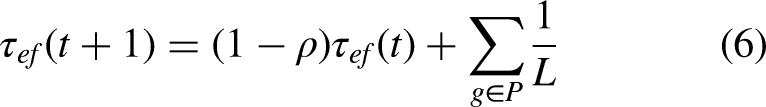 $τ_{e f} (t + 1) = (1 - ρ) τ_{e f} (t) + \sum_{g \in P} \frac{1}{L}$ (6)The parameter $ρ$ is called dissipation coefficient ( $0 < ρ < 1$ ) and $P$ contains all ants passing through segment $e - f$ . L is the total length of the route generated by ant g.

The algorithm stops after $I t_{m a x}$ iterations.

Improved ACO

ACO is characterized by numerous complex mathematical operations that negatively impact its performance, and this is particularly true when the dimensions of the environmental model are large to include significant details. For this reason, various modifications to this algorithm can be found, focused on simplifying such operations. This article proposes the modifications explained below.

Pheromone map simplification: The pheromone map is generally represented as a multidimensional matrix dependent on the possible segments to go through the ants. After the environment modeling, the terrain is limited to a set of cells that can be used as pheromones carriers.²² So, the pheromone map transforms into a bidimensional array of a size equivalent to the environment model. The notation $τ_{e f}$ is reduced to $τ_{f}$ . Reducing the pheromone map significantly decreases the number of mathematical operations required in each iteration, reducing computational load and execution time.

Free step length: The original ACO sets the step length to the distance between two adjacent cells, which reduces candidate cells and search diversity. To avoid these problems, a free step length²³ is adopted. Define visual range (VRange) as the largest range to make an immediate movement without collisions and, as visual field, the set of all cells in the visual range that actually can be reached in a single move. For example, in Figure 4, the circle can be set as the visual range, but the gray cells are not in the visual field because obstacles block them.

Figure 4.

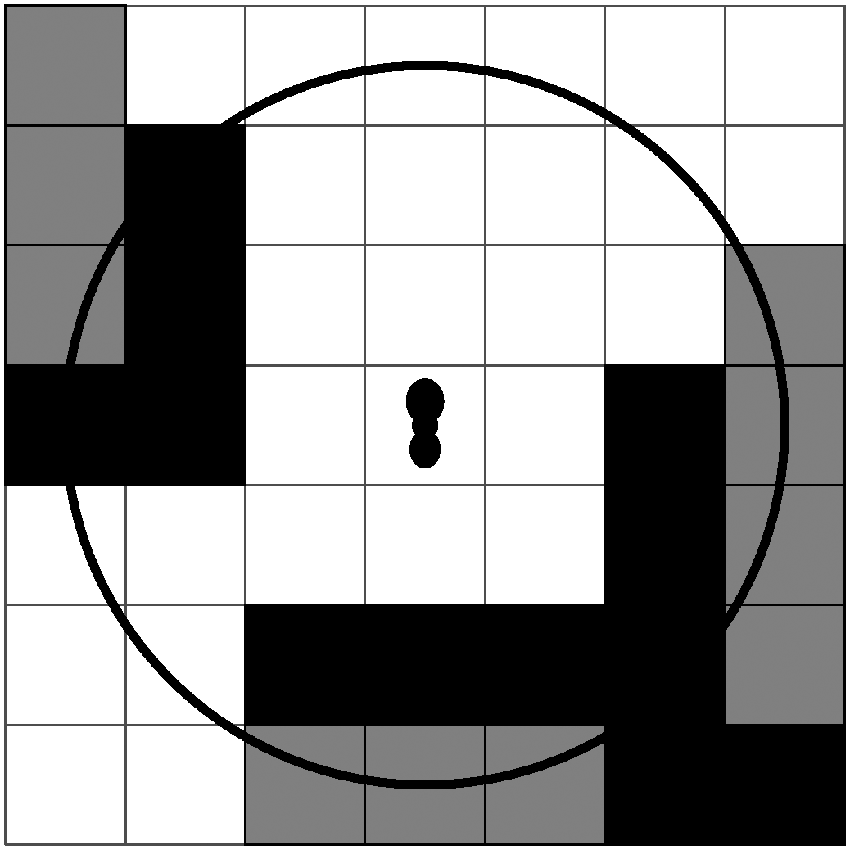
Visual range and visual field.

Following the allowed movement directions, the ant can move to any cell in its visual field.

With a free step length inclusion, ants gain a broader environment sense. A maximum movement simultaneously minimizes the distance to the destination point should be preferred. Therefore, $ν_{e f} (t)$ will be calculated as a division, where the numerator represents the distance between e and f and the denominator, the distance between f and the vehicle’s final position.

The inclusion of the free step length enhances the convergence capabilities and speed of the algorithm. Each ant step is determined by visibility and probability calculations, where the number of possible steps significantly influences the required processing and execution time. A broad visual range dramatically decreases the number of steps, reducing the chance of selecting inappropriate routes. However, by limiting candidate cells to the eight movement directions, there is a drawback of potentially overlooking promising routes.

The proposed ACO algorithm, adapted as described, is called improved ant colony optimization (IACO).

Path correction

Finding correct paths based on exploring a solutions space instead of deterministic rules can significantly reduce effort, especially when that rules incorporate complex mathematical developments. However, the search methods imply that solutions can be improved in some cases, especially in ample search space. For paths made up of straight line segments, it is possible to devise some correction schemes, such as removing redundant nodes.¹⁵ This procedure considers the possibility that the route length can be shortened by connecting two nodes with an obstacle-free line of sight between them. Intermediate nodes are removed.

Results

To check the algorithms strength in path planning, simulated experiments are accomplished in the Matlab software tool. The selected variables to evaluate the performance are the total execution time until a suitable path is reached and the path length value.

The generation methods were executed 500 times in three distinct environments to mitigate randomness in the data. The original methods are also included in the simulation for the purpose of comparing their statistics with those of the improved versions.

The environments differ in obstacles number and the distributions they have:

Environment 1. This environment is the least complex of the three used. It has only one obstacle.

Environment 2. This environment presents a moderate complexity. It has five obstacles with regular shapes.

Environment 3. In this environment, the number of obstacles and their geometric complexity increase. It presents eight obstacles with various shapes.

Each named environment is modeled as a map of

100 \times 100

cells. The vehicle starts its path near the upper left corner of the terrain and ends near the lower right corner.

The initial calibration of the design parameters is done according to the guidelines established in the bibliography.^23,24 From there, it is adjusted by empirical procedures. Table 1 shows the selected parameters. Regarding the dynamic parameters of ENHS, the table presents the boundaries within which the algorithm operates, guided by the rules illustrated in Figure 2.

Table 1.

Algorithm parameters chosen for the simulated experiments.

	HS			ENHS
	Env. 1	Env. 2	Env. 3	Env. 1	Env. 2	Env. 3
$I t_{m a x}$	30,000	30,000	2,000,000	30	100	200
HMS	50	50	50	50	50	50
NHMS	–	–	–	400	400	6000
HMCR	0.77	0.77	0.95	0.7–0.95	0.7–0.95	0.7–0.95
PAR	0.1	0.01	0.01	0.05–0.1	0.1–0.3	0.1–0.3
BW	5	5	5	5–40	5–40	5–40
GBR	–	–	–	0.8	0.8	0.8
D	–	–	–	10	10	20
$ω_{c}$	1	1	1	1	1	1
$ω_{l}$	0.0001	0.0001	0.0001	0.0001	0.0001	0.0001

	ACO			IACO
	Env.1	Env. 2	Env. 3	Env. 1	Env. 2	Env. 3
NoAnts	20	20	20	35	20	20
NoTime	50	50	50	45	50	50
VRange	–	–	–	25	25	25
$α$	1	1	1	1	1	1
$β$	6	6	6	6	6	6
$ρ$	0.3	0.3	0.3	0.1	0.3	0.3

Env.: environment; HS: harmony search; ENHS: enhanced harmony search; HMS: harmony memory size; NHMS: new harmony memory size; HMCR: harmony memory consideration rate; PAR: pitch adjustment rate; BW: bandwidth; ACO: ant colony optimization; IACO: improved ant colony optimization; GBR: global search rate.

Table 2 summarizes the fundamental statistics related to path lengths, providing a detailed overview of the distribution and variability of the results. The statistical measures encompass the minimum ( $l_{m i n}$ ), mean ( $\bar{l}$ ), maximum ( $l_{m a x}$ ), and standard deviation ( $σ_{l}$ ), serving as key indicators to comprehend both the central tendency and data dispersion. Additionally, quartiles are presented, dividing the sample into four equal parts and highlighting values delineating the first, second, and third quartiles ( $Q_{1}$ , $Q_{2}$ , and $Q_{3}$ , respectively). The path length is represented in units referring to the number of cells it occupies (u). The information pertaining to mean execution time ( $\bar{t}$ ) and temporal standard deviation ( $σ_{t}$ ) obtained is also recorded. The unit of time employed is the second (s).

Table 2.

Statistical results derived from the simulated experiments.

	HS			ENHS
	Env. 1	Env. 2	Env. 3	Env. 1	Env. 2	Env. 3
$l_{m i n}$	137.93	170.14	171.52	137.93	168.99	175.96
$\bar{l}$	140.98	173.95	184.64	139.70	171.24	184.76
$l_{m a x}$	143.14	192.92	213.49	141.49	180.72	187.99
$σ_{l}$	1.14	3.14	4.44	0.75	1.87	2.32
$Q_{1}$	140.02	171.95	182.38	139.29	170.30	183.69
$Q_{2}$	141.38	173.00	213.87	139.98	170.80	185.23
$Q_{3}$	142.13	174.79	187.31	140.08	171.47	186.40
$\bar{t}$	0.02	0.93	79.56	0.02	0.87	19.24
$σ_{t}$	0.01	0.07	88.05	0.02	0.19	26.90

	ACO			IACO
	Env.1	Env. 2	Env. 3	Env. 1	Env. 2	Env. 3
$l_{m i n}$	137.43	169.92	175.79	139.64	175.69	192.10
$\bar{l}$	138.68	175.67	189.12	142.15	183.46	203.58
$l_{m a x}$	143.81	194.02	201.52	142.68	189.58	215.15
$σ_{l}$	0.86	4.27	6.97	0.68	2.68	4.22
$Q_{1}$	137.93	172.62	185.42	141.88	181.61	200.52
$Q_{2}$	138.37	174.56	188.56	142.50	183.62	203.41
$Q_{3}$	139.29	177.69	193.12	142.68	185.34	206.69
$\bar{t}$	9.01	181.18	321.48	0.75	1.90	2.83
$σ_{t}$	0.58	52.48	50.56	0.04	0.34	0.26

Env.: environment; HS: harmony search; ENHS: enhanced harmony search; ACO: ant colony optimization; IACO: improved ant colony optimization.

Figure 5 shows the best path generated by ENHS and IACO in the three scenarios discussed.

Figure 5.

Generated paths: (a) ENHS—Environment 1; (b) ENHS—Environment 2; (c) ENHS—Environment 3; (d) IACO—Environment 1; (e) IACO—Environment 2; and (f) IACO—Environment 3. ENHS: enhanced harmony search; IACO: improved ant colony optimization.

Discussion

Firstly, examine the compelling evidence indicating the enhanced performance of the modified algorithms compared to their original counterparts. Table 2 showcases time statistics for HS and ACO, marked in bold style, revealing values exceeding fourfold those observed in ENHS and IACO, respectively. Excessively high processing times are disadvantageous when selecting a candidate algorithm for implementation in the AGV’s path planning module because it can impact the response of subsequent navigation and tracking systems. The benefits of improvements are consistently evident in ACO across diverse scenarios. In the context of HS, the impact of enhancements becomes particularly notable in the high-complexity scenario.

According to the optimal length results shown in Table 2, the two algorithms have the goodness of correctly minimizing the distance if a sufficiently large iterations number is allowed. In terms of execution time performance, both methods exhibit statistics within ranges relatively similar to projects documented in the literature, even when employing different approaches (no metaheuristics) in path planning. This observation is supported by the data presented in Table 3, which compares the results obtained in this study with several projects reported in the specialized literature, developed in environments of similar complexity. Projects that use models of scenarios equivalent to those used in this article have been selected, thus ensuring the validity and relevance of the comparison made.

Table 3.

Comparison of execution time results with other projects collected in the literature. Unit of measurement: seconds.

Reference	Path planingapproach	Optimization criteria	Environmentcomplexity	Processing time
This paper	ENHS	Shorter safe path.	Low	0.02
This paper	IACO	Shorter safe path with movement constraints.		0.75
Santos et al.²⁵	Modified cell Decomposition with A*	Shortest safe path: – Avoiding excessive roll and pitch angles. – Controlling orientation and limiting maximum robot turn rate.		0.26
Kim et al.²⁶	D* Lite	Shortest safe path.		0.29
This paper	ENHS	Shorter safe path.	Medium	0.87
This paper	IACO	Shorter safe path withmovement constraints.		1.9
Xiaolin et al.¹³	ACO	Shorter safe path withmovement constraints.		4.89
Elhoseny et al.²⁷	GA	Shorter safe path.		0.51
This paper	ENHS	Shorter safe path.	High	26.9
This paper	IACO	Shorter safe path withmovement constraints.		2.83
Xiaolin et al.¹³	ACO	Shorter safe path withmovement constraints.		17.97
Tao et al.²⁸	PRM	Shorter safe path with trajectory conflictresolution for various AGV.		10.59
	IDA*			9.86
	Bug2			9.59

ENHS: enhanced harmony search; IACO: improved ant colony optimization; ACO: ant colony optimization; GA: genetic algorithm.

Despite the aforementioned, several differences between ENHS and IACO emerge in the analysis. For instance, the proposed ENHS provides generated paths with shorter lengths than IACO.

Figure 6 is a graphic presentation of the length data in box plots. The box plot is used to interpret samples in which statistical asymmetry may exist because it decreases the influence of biased values. In each diagram, the box dimension is related to the quartile deviation of the sample and can be interpreted as a dispersion graphic measure. A straight segment inside the box indicates the median value ( $Q_{2}$ ), and the whiskers extend to the extreme data. In addition, crosses in the diagram represented the outliers values.¹³

Figure 6.

Box plots of length data: (a) Environment 1; (b) Environment 2; and (c) Environment 3.

It is essential to point out some atypical data generated in ENHS, whose values exceed the corresponding limits in the box plot. The presence of biased values negatively affects the mean distance and standard deviation measures, indicating that the ENHS results tend to be less consistent than IACO.

Consider the following observations: I.

IACO provides solutions with a larger mean distance and a higher data spread in the simplest environment. In the box plot corresponding to Environment 1, the median and maximum values of IACO are very close, implying that approximately 50% of the executions return the biggest solutions. On the other hand, ENHS presents lower mean, median, and sample dispersion values. Furthermore, the mean value is less than the median (see Table 2), implying that ENHS is prone to generating minor distance data for this environment.

II.

IACO maintained its behavior in Environment 2, obtaining the longest planned routes and the highest quartile deviation. At the same time, ENHS performs better in reducing path length: it gets a mean distance of 171.24u and a quartile deviation of 0.59u, representing a decrease of 6.6% and 216% concerning the corresponding IACO values.

III.

For the third environment, IACO continues to present the highest values of statistical trends. The mean length obtained by IACO is 203.58, representing an increase of 10.2% compared to the lowest mean value in ENHS. Once again, ENHS presents a mean length value less than the median (see Table 2).

That IACO converges to length values greater than ENHS should not be associated with the fact that a local minimum could not exceed in the optimization process. Instead, the difference can be the result of other factors, such as its movement constraints (Figures 3 and 4).

An excessive delay by the path planning module can negatively influence the performance and stability of the subsequent control modules implemented in the vehicle; therefore, performing an analysis of execution time is essential. Figure 7 contains a graphical representation of the time data from Table 2.

Figure 7.

Execution time.

IACO has a higher mean execution time for the simplest environments. That is expected because node selection probabilities use many computational operations in each iteration. On the other hand, IACO uses only collision-free paths for search, treating the two planning objectives separately. Treatment like this harms, in general, the execution time, but it gives it robustness from path complexity changes. Indeed, the evidence aligns with the empirical reasoning that, in an environment with a high concentration of obstacles, having fewer available free cells for ant movement accelerates the concentration of pheromones on the shortest path. Hence, this type of environment should favor IACO.

The mean execution time in ENHS increases considerably as the environment becomes more complex. For example, the execution time in Environment 3 corresponds to 22 times the value in Environment 2 and more than 1000 times the value in Environment 1. That happens because the HS method includes the two control objectives in the fitness function. So, the expansion of obstacle areas increases the number of invalid solutions and makes it difficult to search in complex environments, forcing the algorithm to repeat itself if it fails to eliminate collisions on the first try. That translates into a more significant expenditure of time and resources.

The large time standard deviation value for ENHS in Environment 3 confirmed the above phenomenon (see Table 2). The time standard deviation in the experiment is related to the frequency at which various failures occur in route generation. If the algorithm fails b times before reaching success, the execution time increases in the order of $(b + 1)$ times. Therefore, more executions with different failures provoke more dispersion in execution time.

In the case of complex environments, it is necessary to consider the precision required by the mission and the dynamics of the guidance and control system. In general, the increase in execution time observed in ENHS is substantially more significant than the reduction in distance achieved concerning IACO. Therefore, IACO is recommended in path planning for complex environments unless the mission’s requirements indicate otherwise.

Conclusion

The path planning task for an AGV is a length minimization and obstacle avoidance problem. This article compares two metaheuristic methods to solve the path planning problem in a bidimensional scenario. A grid method for environment modeling is used, and several simulated experiments are performed in different operating terrains. When studying the optimization strategies, it is noted that the metaheuristic techniques can be successfully adapted to find an optimum route. However, the experiments show that, compared to IACO, ENHS performs better in searching for minor or medium complexity scenarios. As the obstacle zone increases, the performance mentioned above deteriorates quickly; IACO is preferable for highly complex scenarios.

Future work

The results of this study provide valuable guidance for those tasked with selecting a metaheuristic method to implement in a path planning module, considering the anticipated complexity of the environment. As a prospective avenue for further exploration, expanding the conditions of the considered trajectories in experiments is suggested. Investigating the performance of these algorithms in generating paths with specific curvatures or under temporal constraints may be relevant to the specifications of particular research endeavors. Additionally, the consideration of additional parameters, such as variations in environmental density or the presence of dynamic obstacles, could be examined to evaluate the adaptability and robustness of the algorithms across a wider range of scenarios. This diversification of experimental conditions could enhance the understanding of the capabilities and limitations of path planning algorithms in diverse and complex environments.

Footnotes

Declaration of conflicting interests

The author(s) declared no potential conflicts of interest with respect to the research,authorship,and/or publication of this article.

Funding

The author(s) received no financial support for the research,authorship,and/or publication of this article: The authors gratefully acknowledge the financial support provided by CONACHyT through the scholarship awarded to Dizahab Sehuveret Hernández for his graduate studies. This support has been invaluable in facilitating his academic pursuits and contributing to the success of both the ongoing research projects and this article.

ORCID iDs

Dizahab Sehuveret Hernández

Jorge Alberto García-Muñoz

Alejandro I Barranco Gutiérrez

References

Xiangde

Xiang

, et al. Global dynamic path planning algorithm based on harmony search algorithm and artificial potential field method. In: IEEE 6th information technology and mechatronics engineering conference, pp.346–351. DOI: https://doi.org/10.1109/ITOEC53115.2022.9734602.

Quan

Wei

Ouyang

, et al. New harmony search algorithm for mobile robot path planning. In: Yan

Duan

(eds.) Advances in guidance, navigation and control. Singapore: Springer Singapore. ISBN 978-981-15-8155-7, pp.3463–3473.

Xiao

Sun

, et al. Multiobjective path optimization of an indoor AGV based on an improved ACO-DWA. Math Biosci Eng 2022; 19: 12532–12557.

Charis

Lyridis

. A comparative study on ant colony optimization algorithm approaches for solving multi-objective path planning problems in case of unmanned surface vehicles. Ocean Eng 2022; 255. DOI: https://doi.org/10.1016/j.oceaneng.2022.111418.

Bautista-Camino

Barranco-Gutiérrez

Cervantes

, et al. Local path planning for autonomous vehicles based on the natural behavior of the biological action-perception motion. Energies 2022; 15: 1–23.

Candeloro

Lekkas

Sørensen

. A Voronoi-diagram-based dynamic path-planning system for underactuated marine vessels. Control Eng Pract 2017; 61: 41–54.

Kiani

. Adaptive metaheuristic-based methods for autonomous robot path planning: sustainable agricultural applications. Appl Sci 2022; 12: 943–943.

Yan

. Three-dimensional path planning for autonomous underwater vehicles based on a whale optimization algorithm. Ocean Eng 2022; 250: 111070.

. An adaptive environmental sampling path planning technique for autonomous underwater vehicles based on ant colony optimization algorithm. In: IEEE 4th international conference on civil aviation safety and information technology (ICCASIT), 2022. DOI: https://doi.org/10.1109/iccasit55263.2022.9987183.

10.

Al-omoush

Alsewari

Alamri

, et al. Comprehensive review of the development of the harmony search algorithm and its applications. IEEE Access 2019; 7: 14233–14245.

11.

Kumar

Sikander

. An intelligent optimize path planner for efficient mobile robot path planning in a complex terrain. Microsyst Technol 2023; 29: 469–487.

12.

Aghay Kaboli

Selvaraj

Rahim

. Rain-fall optimization algorithm: a population based algorithm for solving constrained optimization problems. J Comput Sci 2017; 19: 31–42.

13.

Xiaolin

Long

Zhang

, et al. Mobile robot path planning based on ant colony algorithm with A* heuristic method. Front Neurorobot 2019; 13: 1–9.

14.

Deng

Zhao

. An improved ant colony optimization algorithm based on hybrid strategies for scheduling problem. IEEE Access 2019; 7: 20281–20292.

15.

Wang

Yang

, et al. Distributed multi-mobile robot path planning and obstacle avoidance based on ACO-DWA in unknown complex terrain. Electronics 2022; 11: 2144.

16.

Mohd

Zhou

. Harmony search algorithm and related variants: a systematic review. Swarm Evol Comput 2022; 74: 101126.

17.

Min-Yuan

Prayogo

Yu-Wei

, et al. A hybrid harmony search algorithm for discrete sizing optimization of truss structure. Autom Constr 2016; 69: 21–33.

18.

Gad

. Particle swarm optimization algorithm and its applications: a systematic review. Arch Comput Methods Eng 2022; 29: 2531–2561.

19.

Wang

Tan

Liu

. Particle swarm optimization algorithm: an overview. Soft comput 2018; 22: 387–408.

20.

Ali

Kareem

Askar

, et al. Metaheuristic algorithms in optimization and its application: a review. J Adv Res Electr Eng 2022; 6: 7–12.

21.

Agrawal

Sudheer

Ashok

. Ant colony based path planning for swarm robots. In: Proceedings of conference on advances in robotics. AIR ’15, Goa, India: ACM. ISBN 978-1-4503-3356-6, pp.611–615. DOI: https://doi.org/10.1145/2783449.2783511.

22.

Wang

Kan

Guo

, et al. 3D path planning for the ground robot with improved ant colony optimization. Sensors 2019; 19: 815.

23.

Akka

Khaber

. Mobile robot path planning using an improved ant colony optimization. Int J Adv Rob Syst 2018; 15: 1–7.

24.

Kougias

Theodossiou

Kakoudakis

, et al. Harmony search algorithm, a novel optimization technique. Parameter calibration and applications on water resources management problems. In: Proceedings of international CEMEPE & SECOTOX conference. Skiathos, Grecia, pp.245–250.

25.

Juman

Wong

Rajkumar

, et al. An integrated path planning system for a robot designed for oil palm plantations. In: TENCON 2017-2017 IEEE region 10 conference. pp.1048–1053. https://doi.org/10.1109/TENCON.2017.8228012 https://doi.org/10.1109/TENCON.2017.8228012 .

26.

Kim

Hai

Joe

. A guide to selecting path planning algorithm for automated guided vehicle (AGV). In; Duy

Dao

Zelinka

, et al. (eds.) AETA 2017 - recent advances in electrical engineering and related sciences: theory and application. Cham: Springer International Publishing, pp.587–596. https://doi.org/10.1007/978-3-319-69814-4_56 https://doi.org/10.1007/978-3-319-69814-4_56 .

27.

Elhoseny

Tharwat

Hassanien

. Bezier curve based path planning in a dynamic field using modified genetic algorithm. J Comput Sci 2018; 25: 339–350.

28.

Tao

Daichuan

Weifeng

, et al. A novel integrated path planning algorithm for warehouse AGVs. Chin J Electron 2021; 30: 331–338.