Sage Journals: Discover world-class research

Abstract

The path planning for an Unmanned Aerial Vehicles ensures that a dynamically feasible and collision-free path is planned between a start and an end point within a navigation environment. One of the most used algorithms for path planning is the Rapidly exploring Random Tree, where each one of its nodes is randomly collected from the navigation environment until the start and end navigation points are connected through them. The Rapidly exploring Random Tree algorithm is probabilistically complete, which ensures that a path, if one exists, will be found if the quantity of sampled nodes increases infinitely. However, there is no guarantee that the shortest path to a navigation environment will be planned by Rapidly exploring Random Tree algorithm. The Rapidly exploring Random Tree* algorithm is a path planning method that guarantees the shorter path length to the UAV but at a high computational cost. Some authors state that by informing sample collection to specific positions on the navigation environment, it would be possible to improve the planning time of this algorithm, as example of the Rapidly exploring Random Tree*-Smart algorithm, that utilize intelligent sampling and path optimization procedures to this purpose. This article introduces a novel Rapidly exploring Random Tree*-based algorithm, where a new sampling process based on Sukharev grids and convex vertices of the security hulls of obstacles is proposed. Computational tests are performed to verify that the new sampling strategy improves the planning time of Rapidly exploring Random Tree*, which can be applied to real-time navigation of Unmanned Aerial Vehicles. The results presented indicate that the use of convex vertices and grid of Sukharev accelerate the planning time of the Rapidly exploring Random Tree* and show better performance than the Rapidly exploring Random Tree*-Smart algorithm in several navigation environments with different quantities and spatial distributions of polygonal obstacles.

Keywords

Path planning RRT*sampling convex vertices Sukharev grids

Introduction

One of the major advantages of automatic path planning capability for an Unmanned Aerial Vehicle (UAV) is the increase of safety for the vehicle itself. If a communication problem occurs in a remotely controlled telemetry UAV system, the vehicle can detect such a fault with the control station and plan a safety path to navigate to a location that allows communication to be restored. In a situation where there is a permanent loss of communication system, such as damage in radio antenna, the UAV can plan a path to a safe place for an attempt to land, avoiding the exposure of people to the risks of this landing procedure. Another advantage would be the ability of an UAV to adapt itself to changes in a previously planned mission, planning paths to its navigation to accomplish new tasks. Reviews on development and applications of UAV path planning are available on the literature.^1,2

Automatic path planning is a complex problem due to: the avoidance requirement of air exclusion zones (no-fly zones); the avoidance requirement of collision situations with obstacles; and the kinematics and dynamics constraints of the vehicle. This problem can also be observed with another type of vehicles, such as unmanned ground vehicles,^3,4 unmanned surface vehicles,^5,6 and underwater vehicles.^7,8 In this problem, a dynamically feasible path must be planned between a start point and an end point of a navigation environment, allowing the vehicle to navigate, avoiding air exclusion zones and collision situations with obstacles in that environment. The path planning consists of three main steps: the computational modeling of a navigation environment; the planning of a collision-free navigation path; and the conversion of this path into a dynamic feasible path.^1,9

With the increasing capacity of processing and storage of computational data into ever smaller and cheaper devices and with the greater industrial and military interest, the path planning problem has been widely explored. Different abstractions and solutions for path planning have been proposed, among them a class of solutions are called sampling-based algorithms. In this class of algorithms, the navigation environment is not explicitly represented by the algorithm itself. Instead, samples of the navigation environment are collected to compose your solution. To verify if a collected sample generates a collision situation, these algorithms use a collision module responsible for this verification. This class of algorithms is popular in large part because of its computational efficiency and simplicity.

Probabilistic RoadMaps (PRM) ¹⁰ and Rapidly exploring Random Trees (RRT) ¹¹ are the sampling algorithms most applied to the problem of automatic path planning. Both are probabilistically complete, that is, if there is a solution, the chance of the algorithm finding it approaches the value one, as the number of samples collected increases. RRT is an algorithm based on a tree graph, in which samples of the navigation environment are collected randomly. Each collected sample is added to the closest node of the tree, if the straight line, formed by those nodes, is collision free. The tree is expanded until a path between the start and the end navigation points for the UAV is planned.

Although RRT is probabilistically complete, there is no guarantee that the solution found will be a path with an approximate length of the shortest path (optimal solution) length for a given navigation environment. Some solutions were proposed with the objective of achieving this characteristic. These algorithms are asymptotically optimal, which means that the best path can be obtained by them as a solution, preventing the number of samples tends to infinity. Examples of these algorithms are rapidly exploring random graph (RRG)¹² and RRT*.¹³ RRT* algorithm incorporates asymptotic optimality to the RRT algorithm. In RRT*, for each new node added to the tree, its neighborhood of nodes is generated with a given radius distance. Different from the standard RRT algorithm, the new sampled node is not added to the nearest node. Instead, the new sampled node is added to its neighbor node that provides the shorter path length to the root node (navigation starting point). Next, it is verified if the other nodes of its neighborhood can be reconnected with this new node to reduce the length of the path between them and the navigation root node. Thus, when a complete path is planned, it is expected to obtain the shortest path between the root node and the final navigation point. Therefore, there is a larger probability that the navigation path planned by the RRT* algorithm have a smaller length than the paths planned by the standard RRT.¹³

Its important to note that there are some disadvantages of the RRT* algorithm compared to RRT. Although the RRT* algorithm returns a path of shorter length than the standard RRT, the planning time is considerably longer in the first. That is due to the addition of the process of reconnection of the edges during the tree expansion, which involves additional collision tests to its execution. In addition, the algorithm only ensures that the shortest path is planned if the planning time is infinite, which in real path planning applications cannot be feasible.

There are several works that have proposed solutions to reduce the convergence time of the RRT* solution applied to the planning of navigation paths. In these works, heuristics/strategies are used to bias the sampling process of RRT and RRT*, prioritizing sampling of new nodes in certain regions of the navigation environment. Among these works, we can mention Multi-Sample (MS-RRT), ¹⁴ RTT Voronoi Diagram based, ¹⁵ Goal-oriented test generation RRT based, ¹⁶ RRT*-Smart, ¹⁷ Selective Retraction-based RRT, ¹⁸ Poisson RRT, ¹⁹ Potential Guided Directional-RRT* (P-RRT*), ²⁰ Sampling probabilities and fuzzy logic RRT based, ²¹ Informed-RRT*.²²

The contribution of this work is the study of the use of two different sampling strategies in the RRT*: the spatial distributions of samples based on Sukharev grids⁹; and the application of samples defined by the convex vertices of the safety hulls of navigation environment obstacles. The safety hull is a region that confines the whole body of an obstacle, with its vertices defined at a certain safety distance from the obstacle edges. It is generated to use in cases where the vehicle exceeds its limits, avoiding collisions with the real limits of the obstacle. A new algorithm is proposed in this work to study these two sampling strategies: RRT* Sukharev vertices (RRT*-SV). The purpose of using these two sampling strategies is to accelerate the planning of the shortest path possible in a minor planning time. The significant improvement of the RRT*-SV is demonstrated by means of statistical comparison between its results with those obtained with the RRT* and RRT*-Smart algorithms, when applied to path planning in navigation environments with different spatial distribution and arrangement of static obstacles. The RRT*-Smart algorithm was selected, among the works listed in the bibliographic review, due to its efficiency and by having a sampling method that also aims to the planning of paths of shorter length. The RRT* algorithm was selected because it is the basic strategy of the RRT*-Smart and RRT*-SV algorithms.

This work is structured as follows: in the second section, the RRT and RRT* algorithms are described; the third section presents the RRT*-Smart algorithm; in the fourth section, the concept of a Sukharev grid is presented; in the fifth section, the use of convex vertices of the safety hulls of obstacles is discussed; in the sixth section, the RRT*-SV algorithm is introduced; in the seventh section, the results of the simulations between RRT*, RRT*-Smart and RRT*-SV are described and analyzed; in the eighth section, conclusions and future work are discussed.

RRT and RRT* algorithms

The RRT algorithm for path planning is described in Algorithm 1. RRT algorithm constructs a tree that explores the navigation environment Q until a navigation path is planned between an initial position $q_{i n i t}$ and a final position $q_{g o a l}$ . Q represents the set of points/positions of a navigation environment. Q is divided into two subsets: $Q_{f r e e}$ , representing the navigable regions of the navigation environment, that is, the regions without obstacles; and $Q_{o b s}$ , the spatial representation of the obstacles. The main procedures of the algorithm are defined as follows: rand_config: generate a random position $q_{r a n d}$ in the Q navigation environment; nearest_node: search the node $q_{n e a r}$ of G closest to $q_{r a n d}$ ; and new_config: generate a new sample $q_{n e w}$ on the line segment $\bar{q_{n e a r} q_{n e w}}$ at a distance $Δ q$ from $q_{n e a r}$ . If the straight-line segment $\bar{q_{n e a r} q_{n e w}}$ is collision-free, then the following procedures are also performed: extend: expand the tree by assigning $q_{n e a r}$ as the predecessor/parent node of $q_{n e w}$ and adds $q_{n e w}$ to G; and route: collect all nodes that connect $(q_{g o a l} \in Q_{f r e e})$ (final position) to $(q_{i n i t} \in Q_{f r e e})$ (initial position) forming the R route.

Algorithm 1.

RRT algorithm.

The algorithm works by expanding the tree G randomly from the root node $q_{i n i t}$ until one of its branches reaches the final point $(q_{g o a l} \in Q_{f r e e})$ of the path to be planned, or until a maximum number of iterations $(n)$ is reached. At each iteration of the algorithm, leaf node $q_{n e w}$ is added to expand G. In the procedure to create $q_{n e w}$ , $q_{r a n d} \in Q$ is randomly sampled from the navigation environment. The node $q_{n e a r} \in G$ closest to $q_{r a n d}$ is then selected to expand G. The sample $q_{n e w}$ is created to a distance $Δ q$ from $q_{n e a r}$ over the straight line segment $\bar{q_{n e a r} q_{r a n d}}$ . If the straight line segment $\bar{q_{n e a r} q_{n e w}}$ is collision-free, that is, if this line segment does not intercept any obstacle of $Q_{o b s}$ , then $q_{n e w}$ is added to G, such that $q_{n e a r}$ is the predecessor of $q_{n e w}$ . If the distance between this new node $q_{n e w}$ and $q_{g o a l}$ is smaller than the parameter l_d and the straight line segment $\bar{q_{n e w} q_{g o a l}}$ is collision-free, then $q_{g o a l}$ is added to G, such that $q_{n e w}$ is the predecessor of $q_{g o a l}$ ; and the path is planned by storing, in a stack R, each predecessor node from $q_{g o a l}$ until $q_{i n i t}$ , and the algorithm is terminated ( $s = 1$ ).

Several extensions of the RRT algorithm have been published over the years: adaptative RRT based on Dynamic Step (DRRT),²³ RRT Star (RRT*),¹³ Fast RRT,²⁴ Real-time Closed-loop RRT (CL-RRT)²⁵ and its derivation Closed-loop Random Belief Trees (CL-RBT),²⁶ Resolution Complete RRT (RC-RRT),²⁷ Execution extended RRT (ERRT),²⁸ Chance-Constraint RRT (CC-RRT),²⁹ CC-RRT*-D,³⁰ RRT-Connect,³¹ among others. Therefore, the variability of studies focused on improving or adapting some aspect of the RRT algorithm is remarkable.

The difference between the RRT algorithm and the RRT* is in the tree expansion mode. During the expansion operation, a path cost function formed to calculate the impact of the addition of a new node is considered. The cost function represents a measure of generic magnitude (depending of the defined restrictions to each path planning problem). In this work, the cost of the path is defined by the accumulation of the Euclidean distance between the nodes of G (resulting in the total length of the path).

The additional RRT* operations are: rrt_star_extend: extend the tree by selecting the neighbor node $q_{n e i g h b o r} \in Q_{n e i g h b o r s}$ that allows to form the path with the smaller length (cost), in comparison with the nodes of $Q_{n e i g h b o r s}$ , from $q_{n e w}$ to $q_{i n i t}$ , passing through $q_{n e i g h b o r}$ ; $Q_{n e i g h b o r s}$ is given by all nodes that are at distance $β (log (n) / n)$ from $q_{n e w}$ , where n is the current quantity of nodes in G; and rewire: $q_{n e w}$ is connected as the predecessor of the neighbor nodes of $Q_{n e i g h b o r s}$ , if they form with it a shorter length path until the $q_{i n i t}$ node.

The cost of a path between any two nodes q_a and q_b of G is defined by

c o s t (q_{a}, q_{b}) = \sum_{i = 1}^{m - 1} c (q_{i}, q_{i + 1})

where m is the quantity of nodes of the path defined by the nodes q_a and q_b; q_i is the ith node of the path between q_a and q_b; $q_{i + 1}$ is the predecessor node of q_i; $q_{1}$ is the last node q_b of the path; q_m is the first node q_a of the path; and $c (q_{i}, q_{i + 1})$ is the cost/length of each pair of consecutive nodes $(q_{i}, q_{i + 1})$ .

For each $q_{n e w}$ , the RRT* algorithm checks if there are no obstacles between it and the $q_{n e a r}$ node selected. If it does not, the neighbors nodes of $q_{n e w}$ , within the radius range defined by $β (log (n) / n)$ , are selected and assigned to $Q_{n e i g h b o r s}$ . If $c o s t (q_{i n i t}, q_{n e i g h b o r}) + c (q_{n e w}, q_{n e i g h b o r}) < c o s t (q_{i n i t}, q_{n e a r}) + c (q_{n e w}, q_{n e a r})$ , then this $q_{n e i g h b o r} \in Q_{n e i g h b o r s}$ guarantees the planning of a collision free path to $q_{i n i t}$ shorter than the path connecting $q_{n e a r}$ with $q_{n e w}$ . Thus, each node $q_{n e i g h b o r}$ of $Q_{n e i g h b o r s}$ is analyzed to find the one ( $q_{min}$ ) that allows the shortest path between $q_{i n i t}$ and $q_{n e w}$ . This node $q_{min}$ is then connected to $q_{n e w}$ , such that $q_{min}$ is the predecessor of $q_{n e w}$ . This process is defined in the $r r t_s t a r_e x t e n d$ procedure, as described in Algorithm 2.

Algorithm 2.

Extend procedure of RRT* algorithm.

After defining the shorter path from $q_{i n i t}$ to $q_{n e w}$ , passing through $q_{min}$ , it is verified the possibility of reducing the length of the remaining neighbors of $Q_{n e i g h b o r s}$ . To do this, it is analyzed the length of each path between $q_{i n i t}$ to $q_{n e i g h b o r}$ , passing through $q_{n e w}$ . If $c o s t (q_{i n i t}, q_{n e w}) + c (q_{n e i g h b o r}, q_{n e w}) < c o s t (q_{i n i t}, q_{n e i g h b o r})$ , then the predecessor of $q_{n e i g h b o r}$ is changed to $q_{n e w}$ . In this way, if possible, the path is optimized for all nodes of $Q_{n e i g h b o r s}$ . This process is executed by the procedure $r e w i r e$ , described in Algorithm 3.

Algorithm 3.

Rewire procedure of RRT* algorithm.

RRT*-Smart

RRT*-Smart¹⁷ is an algorithm based on the RRT* algorithm, where two new concepts have been incorporated: path optimization; and intelligent sampling. As presented in Islam et al.,¹⁷ RRT*-Smart has an average time to plan the shortest path lesser than the RRT* algorithm. The RRT*-Smart algorithm is described in Algorithm 4. The additional procedures of the RRT*-Smart algorithm are described as follow: path_optimization: the nodes that form the path from $q_{g o a l}$ to $q_{i n i t}$ visible to each other are directly connected, removing intermediate nodes between them. Visible nodes among each other are those that can form a new collision free edge without the need of intermediate nodes; collect_beacons: the nodes that form the optimized path that connects $q_{i n i t}$ to $q_{g o a l}$ are collected. These nodes, called beacons, are used to force the sampling of points in the navigation environment near them.

Algorithm 4.

RRT*-Smart algorithm.

Path optimization is a strategy based on triangular inequality, where the size of the largest side c of a triangle is always smaller than the sum of the sizes of the others two smaller sides a and b. Therefore, if there are two nodes $q_{p a r e n t_t o_p a r e n t}$ and $q_{n o d e}$ that can be connected directly, without collision, then the intermediate node $q_{p a r e n t}$ between them can be removed from the path. Thus an optimized path length is obtained, since the unnecessary tree edges are discarded. This strategy is described by the Algorithm 5.

Algorithm 5.

Path optimization procedure from RRT*-Smart algorithm.

Intelligent sampling is an approach that uses the nodes of a previously planned path to induce the collection of new samples close to them. When a path is planned, its nodes are stored in $Q_{b e a c o n}$ . These nodes are updated each time a shorter path is planned. Thereafter, a new sample is obtained close to one of the beacons of the last shorter length planned path, when the iteration index i of the planning is equal to a value given by $n + c * b$ , where n is the iteration in which the smart sampling starts, c is an incremental value for each smart sampling execution, and b is a constant that defines how often nodes are sampled from $Q_{b e a c o n}$ . When i does not meet the above condition, the new samples are collected randomly from the navigation environment, as in RRT and RRT*.

Sukharev grid

Sukharev grid is part of a group of point dispersion approaches called low sampling. ⁹ The purpose of these approaches is to allow coverage/sampling of all regions of a navigation environment.⁹ A Sukharev grid achieves the most uniform distribution possible over the navigation environment.

A Sukharev grid is generated to a given quantity of cells k to cover a plane $(ℝ^{2})$ or a space $(ℝ^{3})$ . In this work, the grid is applied to cover the navigation environment $Q \in ℝ^{2}$ . Q is then partitioned into k cells. Each of these cells has a point in the center of its geometry called centroid. In the algorithm proposed in this work, the tree expansion will be done by connecting its leaves/nodes through the centroids of the Sukharev grid cells. The quantity of grid cells per axis of the navigation environment is defined by

⌊ k^{1 / N} ⌋

where N is the dimension of the navigation environment. In Figure 1 an example of the Sukharev grid for $k = 196$ on the $ℝ^{2}$ is shown.

Figure 1.

Distribution of cells generated by the Sukharev grid for k = 196. Font: LaValle.⁹

Convex vertices and path planning

In the representation of the navigation environment through polygons, obstacles are defined by vertices connected by edges that define their limits. Depending on the spatial arrangement between two edges with the same vertex in common, this vertex can be classified as convex or concave. Considering the vertices of a polygonal obstacle ordered clockwise, a vertex v_i of this obstacle is convex, if the sequence $v_{i - 1}, v_{i}, v_{i + 1}$ is clockwise. Otherwise, the vertex is non-convex.

The application of convex vertices in path planning is best known through the visibility graph algorithm.³² A visibility graph allows to plan the shortest path between any two positions in a navigation environment. The idea of the method is to connect the convex vertices of the safety hulls of the obstacles to each other, since they form free collision edges, generating a graph called roadmap. An example of a security hull is shown in Figure 2. In a visibility graph, all mutually visible convex vertices are connected by an edge, that is, all convex vertices are connected if there are collision-free straight-line segments defined by them.

Figure 2.

Example of a security hull (blue) of an obstacle (black) of a navigation environment.

After the construction of the graph, the nodes $q_{i n i t}$ and $q_{g o a l}$ are incorporated to it, connecting them to the convex vertices visible to them, aiming at the planning of different possibilities of paths between $q_{i n i t}$ and $q_{g o a l}$ through these vertices. A visibility graph has the property of allowing the planning of the shortest path between any two nodes, if a method for planning shortest paths in graphs is applied, such as the Dijkstra algorithm.³³ Figure 3 illustrates an example of a shortest path planned with a visibility graph.

Figure 3.

Example of a shortest path (red line) planned in a visibility graph. Font: LaValle.⁹

The development of the algorithm proposed in this work is based on this property of the visibility graphs. In this case, the convex vertices of the safety hulls are considered as elements of $Q_{f r e e}$ .

RRT*-SV algorithm

The algorithm presented in this work, called RRT*-SV (RRT* Sukharev vertices), incorporates two concepts to the RRT* sampling strategy: Sukharev grids and convex vertices of obstacle safety hulls. The path optimization procedure of the RRT*-Smart algorithm is also included on the novel algorithm. RRT*-SV algorithm is described in the Algorithm 6. In comparison to RRT*-Smart, RRT*-SV has the following additional procedures: convex_vertices: obtain all the convex vertices of the navigation environment and store them in $Q_{v e r t i c e s}$ ; vertices_sampling: return the convex vertex that generate a collision-free edge with $q_{n e a r}$ (Algorithm 7); nearest_vertex: search for the nearest convex vertices with respect to $q_{n e a r}$ ; disable_vertex: disable from $Q_{v e r t i c e s}$ the selected vertex as $q_{n e w}$ , that can no longer be connected to any other node; sukharev_grid: generates the Sukharev grid data given the quantity of cells k; sukharev_sampling: generate a new sample of the navigation environment using the Sukharev grid (Algorithm 8); sukharev_cell_diagonal: return the diagonal distance between the centroid/center of a square cell and one of its corners/vertices for the generation of $q_{n e w_t e m p}$ ; sukharev_centroids: return the centroid of the cell containing $q_{n e w_t e m p}$ , if it forms a collision-free edge with it.

Algorithm 6.

RRT*-SV algorithm.

Algorithm 7.

Sampling procedure by convex vertices from RRT*-SV algorithm.

Algorithm 8.

Sampling procedure by Sukharev grid from RRT*-SV algorithm.

In the RRT*-SV sampling process, three attempts are made to generate a new sample to be inserted into the tree. At first one, the algorithm tries to generate $q_{n e w}$ from the convex vertices of the safety hulls of the obstacles of the navigation environment (line 14 of Algorithm 6). If this is not possible, a new attempt is made through the Sukharev grid (line 16 of Algorithm 6). Finally, if it is not possible to generate $q_{n e w}$ after the two attempts with the previous procedures, RRT*-SV tries to get it randomly, as in the standard RRT (line 18 of Algorithm 6). This scenario is illustrated on Figure 4. If after three attempts a new node is not found, a new $q_{r a n d}$ is selected from the tree and all the sampling process is repeated again considering it. A flowchart of the overall behavior of the RRT*-SV algorithm is presented in Figure 5.

Figure 4.

(a) In scenarios where Sukharev centroids or convex vertices are not available to extend the tree, the uniform sampling of the standard RRT algorithm is performed in RRT*-SV. (b) Similar to what occurs in standard RRT, initially a $q_{r a n d}$ sample is generated and then a new sample $q_{n e w}$ is generated given a $Δ q$ distance from its nearest node on the tree $q_{n e a r}$ . (c) If the segment $\bar{q_{n e a r} q_{n e w}}$ is collision free, then $q_{n e w}$ is added to the tree. RRT: Rapidly exploring Random Tree; SV: Sukharev vertices.

Figure 5.

Flowchart of the RRT*-SV behavior. RRT: Rapidly exploring Random Tree; SV: Sukharev vertices.

Further details on the use of each of the strategies proposed in the RRT*-SV algorithm are given in the following subsections. The expected improvements of each is also presented when they are applied as sampling strategies.

Role of convex vertices in the RRT*-SV algorithm

In the process of sampling by convex vertices, each new node sampled from the navigation environment is a convex vertex contained in $Q_{f r e e}$ . These vertices, when added to the tree, are called nodes. In this way, a path is planned near to the obstacle safety hulls, to obtain the shortest path, that is, the optimal solution. The process of sampling by convex vertices is described in Algorithm 7.

In this sampling strategy, $q_{r a n d}$ is generated randomly at each iteration. As in the standard RRT, the tree node $q_{n e a r}$ closest to $q_{r a n d}$ is selected. So, the convex vertex $q_{v n e a r}$ of $Q_{v e r t i c e s}$ closest to $q_{n e a r}$ is searched. These operations are performed by the procedure $n e a r e s t_v e r t e x$ in line 2 of the Algorithm 7. By performance issues, a data structure was used to guide the search for $q_{v n e a r}$ . In this work, $Q_{v e r t i c e s}$ is represented by a k-dimensional (k-d) tree³⁴ structure for this purpose. If the edge joining $q_{n e a r}$ and $q_{v n e a r}$ is collision-free, then $q_{n e a r}$ is connected to $q_{v n e a r}$ , and $q_{v n e a r}$ is eliminated from $Q_{v e r t i c e s}$ , avoiding new uses of this vertex in the sampling process. These steps are illustrated in Figure 6.

Figure 6.

Stages of the sampling process based on convex vertices: (a) a random sample $q_{r a n d}$ is collected and the node $q_{n e a r}$ of G closest to it is obtained; (b) the convex vertex $q_{v n e a r}$ of $Q_{v e r t i c e s}$ closest to $q_{n e a r}$ is searched through a k-d-tree data structure; (c) if the edge connecting $q_{v n e a r}$ and $q_{n e a r}$ is collision free, then $q_{v n e a r}$ is added to the tree as $q_{n e w}$ . Once added to the tree, $q_{v n e a r}$ is not more available for a future sampling.

Collision strategy of the RRT*-SV algorithm

In this work, the obstacles are encapsulated by safety hulls. The distance between the edge of the safety hull and the edge of the obstacle takes into account the size of the vehicle and a safety margin. Thus, the edges and the convex vertices of the safety hulls can be used as structures of a path in the planning process, allowing the safe navigation of the vehicle through them.

Based on these preambles, RRT*-SV algorithm does not verify collision situations between two sequential convex vertices of the same safety hull. However, when two convex vertices of the same safety hull are not sequential or belongs to different hulls, then an edge that connect these two nodes can cause a collision situation with some encapsulated obstacle. These situations are illustrated in Figure 7.

Figure 7.

Example of a valid path between $q_{r a n d}$ and $q_{n e a r}$ in RRT*-SV. Black straight segments are the segments of the path and the black dots are tree nodes or convex vertices that can be added to it. The red edges are examples of possible collisions among convex vertices. RRT: Rapidly exploring Random Tree; SV: Sukharev vertices.

RRT*-SV algorithm uses a collision checker module to verify two types of collision situations: the mentioned collision situations of nodes and edges formed by convex vertices; and the collision situations that can be caused when the sampling is generated through a Sukharev grid, or by an uniform distribution, that is the sampling process of the standard RRT algorithm. In all cases, the collision check process consists in verifying if the edge joining two samples intercepts some safety hull of the navigation environment. There is a collision if there is an intersection, and there is no collision if there is no intersection or if the intersection occurs only with the edge of some safety hull, as explained previously. The structure and relations between the navigation environment, the collision checker module and the sampling strategies of the RRT*-SV algorithm are defined on a diagram block, that is presented in Figure 8.

Figure 8.

Block diagram of path planning by RRT*-SV algorithm. RRT: Rapidly exploring Random Tree; SV: Sukharev vertices.

Role of Sukharev grids in the RRT*-SV algorithm

The centroids of the uniformly distributed cells of the Sukharev grid are used as samples of the navigation environment by the RRT*-SV algorithm. The purpose of using the Sukharev grid is to force the exploration of all navigable regions of the navigation environment, without necessarily sampling all possible points of these regions. Therefore, all the infinite points inside a cell can be represented by a unique point, which is the cell centroid. The expected effects are a smaller number of points sampled to plan a viable path for navigation, to decrease the planning time of a path. The use of Sukharev grids in sampling-based algorithms has already been explored experimentally and theoretically in previous studies.^35
–37 On the context of RRT*-SV, the Sukharev grid sampling process is also useful in situations where it is not possible to connect $q_{n e a r}$ to a convex vertex of $Q_{v e r t i c e s}$ . This occurs when it is not possible to connect a collision-free segment from $q_{n e a r}$ to any convex vertices available for addition to the tree. Figure 9 illustrates an example of this situation.

Figure 9.

Stages of the sampling process based on a Sukharev grid: (a) $q_{r a n d}$ is generated randomly at each iteration; (b) the node $q_{n e a r}$ of G closest to $q_{r a n d}$ is selected; (c) a temporary node $q_{n e w_t e m p}$ is generated at a distance $Δ s$ from $q_{n e a r}$ ; (d) the sample $c e n t r o i d (q_{n e w_t e m p})$ , that is the centroid of the cell containing $q_{n e w_t e m p}$ , is added as the new node $q_{n e w}$ of the tree, if the edge connecting $q_{n e a r}$ to $c e n t r o i d (q_{n e w_t e m p})$ is collision-free. As previously mentioned, this procedure is accomplished if there is not at least one convex vertex that can be connected to $q_{n e a r}$ . Black points are convex vertices. Small brown squares are grid cell centroids generated by the Sukharev distribution.

The process of using a sample of the Sukharev grid, composed by square cells, consists of three steps. In the first step, for a given $q_{r a n d}$ , a sample $q_{n e w_t e m p}$ is generated in the straight line segment $\bar{q_{n e a r} q_{r a n d}}$ , considering a distance $Δ s$ from $q_{n e a r}$ . This step has an equivalent role to the procedure $n e w_c o n f i g$ of the Algorithm 1. The value of $Δ s$ corresponds to the length of the side of a square cell of the Sukharev grid. Thus, the sample $q_{n e w_t e m p}$ is always obtained in the cell containing $q_{n e a r}$ or in one of the cells adjacent to that cell. The parameter k is inversely proportional to the parameter $Δ s$ . The second step is to identify the cell to which $q_{n e w_t e m p}$ belongs. In the third step, it is checked whether the segment formed by the centroid of this cell with the $q_{n e a r}$ node intercepts some security hull. If there is no intersection, the centroid of this cell is stored as a new node ( $q_{n e w}$ ) of the G tree.

Asymptotic analysis of RRT*-SV

Time complexity

The computational time complexity of the RRT*-SV algorithm is based on the complexity of the line 8 and the complexity of the loop of the line 9 of the Algorithm 6. The generation of the Sukharev grid, performed by operation $s u k h a r e v_g r i d$ on line 4, is $O (1)$ , since what is actually generated is the dispersion value of the grid based on equation (2). Using the sizes of the navigation environment axis, the Sukharev cells can be calculated directly through the dispersion value generated. The complexity of the line 8 is $O (n_{t})$ , where n_t is the total number of vertices of all safety hulls of the navigation environment. The calculation of this complexity was based on the asymptotic domain properties described by Ziviani.³⁸ In the worst case, the complexity of the loop of line 9 corresponds to the multiplication of n by the sum of the time complexity of $n e a r e s t_n o d e$ , $v e r t i c e s_s a m p l i n g$ , $r r t_s t a r_e x t e n d$ , and $p a t h_o p t i m i z a t i o n$ . The other components of the loop have complexity $O (1)$ . The first process with significant computational time inside this loop is the search for the nearest node of $q_{r a n d}$ (line 13 of Algorithm 6). It can be found in logarithmic order,³⁹ but in this work was used the brute force strategy for the nearest node search (RRT*, RRT*-Smart and RRT*-SV). So, this process is $O (n)$ , where n is the number of nodes in the tree at the time of the search.

The time complexity of $v e r t i c e s_s a m p l i n g$ (line 14 of Algorithm 6) is equal to the sum of the complexity of $n e a r e s t_v e r t e x$ with the complexity of the collision test. Since n_v is the quantity of convex vertices in $Q_{v e r t i c e s}$ , the procedure $n e a r e s t_v e r t e x$ takes $O (log n_{v})$ on average case and $O (n_{v})$ on the worst case to a k-d-tree structure. The $d i s a b l e_v e r t e x$ do not remove the vertex from $Q_{v e r t i c e s}$ but directly swap its coordinates to the out of the range of the navigation environment, so is $O (1)$ , avoiding the cost of remove it from the k-d-tree. Therefore, $v e r t i c e s_s a m p l i n g$ would cost $O (n_{v}) + O_{c o l l i s i o n}$ in each iteration of the RRT*-SV.

The $r r t_s t a r_e x t e n d$ procedure is based on the neighborhood estimation of $q_{n e w}$ . The quantity of neighbors of $q_{n e w}$ is a portion of the number of nodes in the tree. Thus, the time complexity of $r r t_s t a r_e x t e n d$ is $O (n O_{c o l i s i o n})$ , in the worst case.

As previously described, the $p a t h_o p t i m i z a t i o n$ procedure consists of simplifying a path composed of a portion of nodes in the tree. Then, the time complexity of $p a t h_o p t i m i z a t i o n$ can be calculated to be equal to $O (n O_{c o l l i s i o n})$ .

Finally, the total time complexity of the algorithm is $O (O (n_{t}) + n (O (n) + (O (n_{v}) + O_{c o l l i s i o n}) + O (n O_{c o l l i s i o n}) + O (n O_{c o l l i s i o n}))) = O (O (n_{t}) + n (n O_{c o l l i s i o n} + O (n_{v}) + O_{c o l l i s i o n})) =$ $O (max (O (n_{t}), n (max (n O_{c o l l i s i o n}, O (n_{v})))))$ , in the worst case.

Compared to RRT* and RRT*-Smart algorithms, that have computational complexity equal to $O (n^{2})$ ^13,17 (originally $O (n log n)$ due optimized nearest node search), the RRT*-SV algorithm can demonstrate a different time complexity depending of the value of its additional parameter n_v. If $O (n_{v})$ is lesser than $O (n)$ , the RRT*-SV must show better performance than RRT* and RRT*-Smart algorithms. Otherwise, RRT* and RRT*-Smart must show a better performance instead. The computational tests on the next sections shows this expected behavior.

Computational tests with the RRT*-SV algorithm

Three sets of computational tests were realized aiming the comparison between the RRT*, RRT*-Smart, and RRT*-SV algorithms, the last proposed in this work. The three algorithms were applied to such sets of computational tests and compared considering the planning time and the length of the planned paths. Each set of computational test was elaborated, considering bi-dimensional navigation environments with static obstacles. However, the algorithm can be applied to three-dimensional navigation environments with minor adaptations based on the navigation altitude of the vehicle. The main parameters of the algorithms are described in next subsection. The three sets of computational tests are described in subsequent subsections.

Parameters of the algorithms

This subsection describes the parameter values of the algorithms used in all computational tests. The $Δ q$ parameter was set to 3% of the largest value between the length and height/width of the navigation environment. The distance l_d that defines the distance for the connection check from $q_{n e w}$ to $q_{g o a l}$ was set to 50. The value 6 was set to the b parameter of RRT*-Smart that defines the frequency of use of the beacons generated by the intelligent sampling of this algorithm. The radius $r_{b e a c o n}$ , for the generation of new nodes around a beacon, is equal to 15. The k parameter, that defines the number of Sukharev cells used by RRT*-SV, is equal to 100. The β value, which is used to calculate the radius of the neighborhood search of $q_{n e a r}$ in the RRT*, RRT*-Smart, and RRT*-SV algorithms, was set to 650.

First set of computational tests

Some considerations were made in the first set of computational tests. A single obstacle navigation environment is used, as illustrated in Figure 10. The navigation environment was represented in a Cartesian plane, where the length corresponds to the interval [0.0, 1000.0] in the horizontal axis (X-axis); and the width corresponds to the range [0.0, 1000.0] on the vertical axis (Y-axis). All paths were planned between the initial position (500, 500) and the final position (925, 925), which correspond to $q_{i n i t}$ and $q_{g o a l}$ , respectively. In the three algorithms, a stop condition of 30, 000 iterations was used, and the same seed for generating pseudo-random numbers was used in the random function to generate the samples $q_{r a n d}$ in each simulation. A total of 100 simulations were executed to this computational test. The mean value of the path length planned by each algorithm on these simulations were compared to the optimal path length defined to the navigation environment of this computational test as 1246.

Figure 10.

First set of computational tests (to one simulation): (a) first path planned by RRT* in iteration 457 (non-optmized), (b) by RRT*-Smart in iteration 457, but optimized (red segment), and (c) by the RRT*-SV in iteration 10. The paths planned by the algorithms in the 30, 000 iteration are shown in (d), (e), and (f), respectively. RRT: Rapidly exploring Random Tree.

Considering just one of the simulations as example (which is illustrated in Figure 10), the RRT*-SV algorithm planned a path with length equal to 1246 in the iteration 10. This path corresponds to the optimal solution. Figure 10 illustrates the paths planned by each algorithm to this specific simulation result. Observing the figure cited, it is possible to note that the path planned by the RRT*-SV has a smaller length than the path planned by the other algorithms. The algorithms RRT* and RRT*-SV planned the first path on this result only in the iteration 457. These two algorithms planned the first path in the same iteration because they use the same sampling mechanism until the planning of the first path. However, after planning the first path, the RRT*-Smart algorithm uses a different strategy, based on path optimization through beacons, as previously mentioned.

Through an analysis of Figure 10(a) and (b), it can be observed that the path planned by the RRT*-Smart is the optimized version of the path planned by the RRT*, because the path generated by the first algorithm shares nodes with the path generated by the second, characteristic already presented by Islam et al.¹⁷ This shows that the simulations are in conformation to what is presented by Islam et al.¹⁷

Table 1 presents the average values generated by each algorithm to plan the first path in the 100 simulations with different seeds. RRT*-SV planned the first path, on average, at a run time equal to 0.001 s. The planning time of the RRT* is similar to that of the RRT*-Smart. The first algorithm spent 0.086 s to plan the first path and the second algorithm 0.097 s. The slight difference between these planning times can be assigned to the path optimization procedure of the RRT*-SV. Comparing planning times and lengths, RRT*-SV was 99% faster than RRT*-Smart and still got a 5% shorter path length on average, delivering much better performance in these simulation.

Table 1.

First set of computational tests: average values spent for each algorithm to plan the first path, considering 100 Simulations.

Algorithm	Length	Iteration	Planning time (s)
RRT*	1375	1268	0.086
RRT*-Smart	1316	1268	0.097
RRT*-SV	1255	14	0.001

RRT: Rapidly exploring Random Tree; SV: Sukharev vertices.

In Figure 11, there is a chart of the average length of the paths planned by each algorithm over 30, 000 iterations. It can be observed that the RRT* and RRT*-Smart could not plan the shortest path, that is, the optimal solution (orange horizontal line), in 30, 000 iterations. On the other hand, the RRT*-SV algorithm has planned the near shortest path close to the iteration 2000.

Figure 11.

First set of computational tests: average path length by iteration, considering 100 simulations.

In Figure 12, it is illustrated the chart that represents the iterations in which each algorithm, on average, produces paths that reach or exceed certain fixed values of lengths. There is a large difference in the number of iterations required for each algorithm to achieve the shortest length values. While RRT*-Smart needs 2014 iterations to produce a path of length equal to 1300, a path that was planned by RRT*-SV in 42 iterations had already reached that value. However, it is also necessary to verify the computational time that each algorithm needs to reach each number of iterations, since these algorithms differ significantly in the generation of a new sample of the navigation environment.

Figure 12.

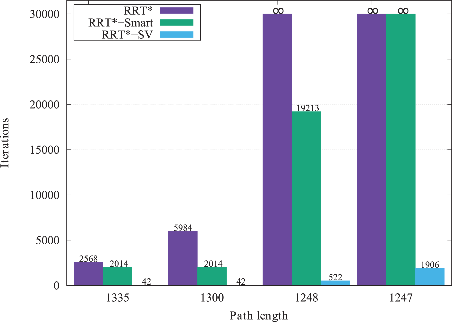
First set of computational tests: average quantity of iterations for each algorithm achieve a specific path length, considering 100 simulations.

Figure 13 presents the chart that relates the computational time required for each algorithm to produce paths that reach or exceed the fixed length values. The planning time of RRT*-Smart to plan a path with length of 1248 was 17.060 s versus a path with length of 0.031 s planned by RRT*-SV. This represents a difference of 99.8% between the planning times, which demonstrates notorious superiority of RRT*-SV over the RRT*-Smart (and consequently over the RRT*) in convergence for a shorter path length and planning time in this computational test.

Figure 13.

First set of computational tests: average planning time for each algorithm achieve a specific path length, considering 100 simulations.

Second set of computational tests

The performance of the RRT*-SV algorithm is dependent of the quantity of convex vertices contained in the navigation environment. The increase of the number of convex vertices implies an increase in the computational complexity of the algorithm RRT*-SV. To analyze the influence of the number of convex vertices on the RRT*, RRT*-Smart and RRT*-SV performance, computational tests were executed using navigation environments with 5, 50, 2500, and 10, 000 obstacles. Each obstacle (and also its safety hull) is a rectangle, resulting in four convex vertices. Then, each navigation environment has, respectively, 20, 200, 10, 000, and 40, 000 convex vertices. For each of these navigation environments, five computational tests were performed with a different seed to generate the $q_{r a n d}$ samples. Also, the tests were accomplished considering 30, 000 iterations. The average values of these test results were used to analyze the performance of the proposed algorithm.

As described in Table 2, RRT*-SV planned the first path faster than RRT* and RRT*-Smart algorithms, considering the navigation environments with 5 and 50 obstacles. In other environments, RRT*-SV planned the first path in a longer run-time, in comparison with the other algorithms. The greater the number of convex vertices, the greater the difference of the time spent by the RRT*-SV algorithm to plan the first path, in comparison with the times spent by the others algorithms also to plan a first path. In the navigation environment with five obstacles, the RRT*-SV algorithm planned a first path at 0.001 s and the RRT*-Smart at 0.039 s, what corresponds to a difference of 97%. In the navigation environment with 50 obstacles, the RRT*-SV planned the first path at 0.010 s and RRT*-Smart at 0.122 s, an advantage of RRT*-SV of 92% over the RRT*-SV. In the 2500 obstacles navigation environment, RRT*-SV planned the first path at 16.617 s, and RRT*-Smart at 4.119 s, so this time RRT*-Smart get advantage of over the RRT*-SV, corresponding to 75%. In the navigation environment with 10, 000 obstacles, the RRT*-SV spent 183.393 s to plan the first path and the RRT*-Smart 42.594 s, a difference of 77% between both algorithms. However, it is important to check the length of the final path planned by each algorithm in each navigation environment. The first paths planned by the RRT*-SV algorithm are presented in Figure 14.

Table 2.

Second set of computational tests: average planning time spent by the algorithms, considering five simulations for each of the four fixed-length values, and considering navigation environments with 5 obstacles, 50 obstacles, 2500 obstacles, and 10,000 obstacles.

RRT*			RRT*-Smart			RRT*-SV
Path length	Iteration	Planning time (s)	Path length	Iteration	Planning time (s)	Path length	Iteration	Planning time (s)
Cluttered 5 obstacles
1495	985	0.018	1452	985	0.039	1780	8	0.001
Cluttered 50 obstacles
1519	1947	0.114	1503	1947	0.122	1492	164	0.0104
Cluttered 2500 obstacles
1589	2961	3.920	1587	2961	4.119	1467	3457	16.617
Cluttered 10000 obstacles
1784	11, 389	40.772	1782	11, 389	42.594	1750	8750	183.393

RRT: Rapidly exploring Random Tree; SV: Sukharev vertices.

Figure 14.

Second set of computational tests: first path planned by RRT*-SV, considering navigation environments with (a) 5, (b) 50, (c) 2500, and (d) 10, 000 obstacles. RRT: Rapidly exploring Random Tree; SV: Sukharev vertices.

Figure 15 presents the chart of the run-time required by each algorithm to produce paths that reach or exceed some fixed-length values, considering four configuration of navigation environments. In Figure 15(a) and (b), the RRT*-SV presents planning time smaller than the planning times of the other algorithms to reach the fixed lengths. In Figure 15(c) and (d), it can be seen that the RRT*-SV only gains advantage over the other algorithms considering the last fixed path lengths of 1369 and 1410, respectively (RRT* and RRT*-Smart were unable to plan paths with these fixed-length values). This fact implies that, even for navigation environments with high quantities of obstacles, RRT*-SV can converge more quickly to better solutions.

Figure 15.

Second set of computational tests: information about the first paths planned by the algorithms, considering navigation environments with 5, 50, 2500, and 10,000 obstacles.

Therefore, for this second set of computational tests, it is concluded that RRT*-SV tends to converge more quickly to shortest paths than RRT*-Smart, and consequently, than RRT*. However, in navigation environments with many obstacles (2500 and 10, 000 obstacles), RRT*-SV algorithm tends to have a higher run-time to plan a first path. Therefore, it is suggested to use each algorithm depending on the requirements and characteristics of the path planning problem to be explored. In navigation environments with high quantity of obstacles, if a path must to be planned in the shortest time possible, RRT*-SV cannot be the most appropriate. However, if the requirement is to obtain a path with minimized length, the RRT*-SV offers advantage over the other algorithms analyzed in this work.

Third set of computational tests

In this section, it is described a set of computational tests aiming to a statistical comparison between the RRT*-Smart and the RRT*-SV algorithms by means of the statistical method denominated t Student.⁴⁰ Fifteen simulations were executed considering navigation environments with different spatial distributions of obstacles. The specifications of the values of $q_{i n i t}$ and $q_{g o a l}$ for each of these navigation environments are described to follow: $q_{i n i t} = (25, 25), q_{g o a l} = (975, 975)$ for a navigation environment with five obstacles; $q_{i n i t} = (25, 25), q_{g o a l} = (975, 975)$ for a navigation environment with 50 obstacles; $q_{i n i t} = (25, 25), q_{g o a l} = (975, 975)$ for a navigation environment with 100 obstacles; $q_{i n i t} = (25, 25), q_{g o a l} = (975, 975)$ for a navigation environment with 200 obstacles; $q_{i n i t} = (500, 50), q_{g o a l} = (500, 950)$ for a navigation environment with a set of obstacles placed in zig-zag; $q_{i n i t} = (500, 500), q_{g o a l} = (500, 100)$ for a navigation environment with an U-shape obstacle; $q_{i n i t} = (25, 25), q_{g o a l} = (940, 940)$ for a navigation environment with a maze shape; $q_{i n i t} = (500, 500), q_{g o a l} = (925, 925)$ for a navigation environment with obstacles in a spiral shape; and $q_{i n i t} = (25, 25), q_{g o a l} = (925, 925)$ for a navigation environment with obstacles forming a narrow passage. The paths planned by the RRT*-SV algorithm in these navigation environments are illustrated in Figure 16.

Figure 16.

Third set of computational tests: paths planned by the RRT*-SV algorithm, considering different configurations of navigation environments: (a) 5 obstacles; (b) 50 obstacles; (c) 100 obstacles; (d) 200 obstacles; (e) Maze; (f) Zigzag; (g) Spiral; (h) Narrow passage; and (i) U-form.RRT: Rapidly exploring Random Tree; SV: Sukharev vertices.

To define the quantity of simulations, the confidence interval (CI) was calculated for each of the computational tests, considering the nine navigation environments described previously. The CI value estimates an interval containing the hypothetical population mean at a given confidence level assuming that the results of the algorithms in the computational tests follows a normal distribution. The estimate of CI was calculated with 95% confidence level, which in the normal distribution corresponds to $z = 1.45$ . The smaller the range amplitude, the better the chances of the real average be contained in this interval with the specified confidence level. The range is affected by the quantity of samples collected. It was considered that the calculated intervals allow to infer that the number of simulations performed is adequate for the statistical analysis. The statistical variables considered in this analysis were the length of the planned path and its planning time. The CI values for each navigation environment are described in Table 3.

Table 3.

Third set of computational tests: application of the t student method to statistically compare the results obtained by the planning algorithms, considering 15 simulations for each navigation environment.

		Path length					Planning time (s)
Algorithm	Iterations	Average	Std Dev.	CI	t Value	z	Average	Std Dev.	CI	t Value	z
Cluttered 5 obstacles
RRT*-Smart	5000	1417	4	1417 ± 2	3.451	2.048	0.451	0.201	0.451 ± 0.101	−3.121	2.048
RRT*-SV	5000	1413	1	1413 ± 0	3.451	2.048	0.784	0.362	0.784 ± 0.183	−3.121	2.048
Cluttered 50 obstacles
RRT*-Smart	5000	1438	22	1438 ± 11	7.214	2.048	0.564	0.274	0.564 ± 0.139	−4.062	2.048
RRT*-SV	5000	1397	6	1397 ± 3	7.214	2.048	1.05	0.374	1.05 ± 0.189	−4.062	2.048
Cluttered 100 obstacles
RRT*-Smart	5000	1438	24	1438 ± 12	9.29	2.048	0.656	0.21	0.656 ± 0.106	−4.397	2.048
RRT*-SV	5000	1379	4	1379 ± 2	9.29	2.048	1.925	1.098	1.925 ± 0.556	−4.397	2.048
Cluttered 200 obstacles
RRT*-Smart	5000	1533	45	1533 ± 23	10.709	2.048	0.945	0.412	0.945 ± 0.208	−4.287	2.048
RRT*-SV	5000	1406	10	1406 ± 5	10.709	2.048	2.994	1.804	2.994 ± 0.913	−4.287	2.048
U-form
RRT*-Smart	5000	1385	12	1385 ± 6	2.665	2.048	0.473	0.177	0.473 ± 0.09	−3.737	2.048
RRT*-SV	5000	1377	0	1377 ± 0	2.665	2.048	1.148	0.677	1.148 ± 0.342	−3.737	2.048
Spiral
RRT*-Smart	7000	2349	29	2349 ± 15	6.138	2.048	0.611	0.33	0.611 ± 0.167	−4.06	2.048
RRT*-SV	7000	2302	0	2302 ± 0	6.138	2.048	1.543	0.826	1.543 ± 0.418	−4.06	2.048
Zigzag
RRT*-Smart	5000	1154	57	1154 ± 29	10.108	2.048	0.599	0.271	0.599 ± 0.137	−3.001	2.048
RRT*-SV	5000	1006	0	1006 ± 0	10.108	2.048	1.324	0.895	1.324 ± 0.453	−3.001	2.048
Maze
RRT*-Smart	10,000	1802	3	1802 ± 1	15.62	2.048	1.642	0.543	1.642 ± 0.275	−4.821	2.048
RRT*-SV	10,000	1790	0	1790 ± 0	15.62	2.048	3.792	1.64	3.792 ± 0.83	−4.821	2.048
Narrow passage
RRT*-Smart	25,000	1588	2	1588 ± 1	17.358	2.048	7.968	1.57	7.968 ± 0.795	0.645	2.048
RRT*-SV	25,000	1581	0	1581 ± 0	17.358	2.048	7.62	1.388	7.62 ± 0.702	0.645	2.048

RRT: Rapidly exploring Random Tree; SV: Sukharev vertices; CI: confidence interval; std dev.: standard deviation.

In this third set of computational tests, statistical variables were modeled as random, without autocorrelation between the results of each simulation for each method and without dependence between RRT*-Smart and RRT*-SV results. To compare them, t Student method was applied to verify the null hypothesis, in other words, to test if there is no difference between the two sets of samples (computational test results). If the null hypothesis is considered true, there will be no significant difference between the sample means. Otherwise, the test identifies the difference and shows how significantly both differ. The test is adequate when the averages and population variances from which the samples were taken are not known.⁴¹ The version of t Student method used was Welch’s unequal variances t test,⁴² applied when the variances between the two samples are different. The value of α was set equal to 0.05 in this third set of computational tests.

Based on the results presented in Table 3 for the statistics about the length of the planned paths at the end of the simulation iterations, in the computational tests with the RRT*-SV, the average length of the paths was shorter, for all navigation environments considered, than the average length of the paths obtained in the computational tests with the RRT*-Smart algorithm. Moreover, the standard deviations of RRT*-SV averages are smaller when compared to the standard deviations obtained by the RRT*-Smart, that is, the lengths of the paths obtained with RRT*-SV are smaller and vary less than those planned by the RRT*-Smart, for the quantity of iterations considered. The values of the t Student method were higher than the values of z, which by the test criteria indicates that the null hypothesis is false, and that the methods present a difference between their results.

Analyzing the data of Table 3, RRT*-SV does not present the best performance, considering the statistical data generated for the planning time. The navigation environment with a narrow passage is the unique case where the algorithm has no statistical difference in relation to the RRT*-Smart, since the absolute value of t value was not greater than the value of z. Therefore, the null hypothesis cannot be discarded to this navigation environment. For the others navigation environments, the RRT*-Smart planning time was lower than the RRT*-SV planning time, considering the total quantity of iterations applied to each of them. However, it is worth mentioning that despite the worst performance in planning time of the RRT*-SV for some of these navigation environments, the final path length obtained by it is still shorter.

The idea of using the convex vertices in the RRT* sampling process is to accelerate convergence to a solution of the algorithm. To assist in the hypothesis that this will occur, t Student method was also performed considering only the simulation data related to the first path planned by each algorithm.

The statistics related to the first planned paths on the simulations are described in Table 4. In the navigation environment with five obstacles, RRT*-Smart obtained better performance than RRT*-SV for the planning of shorter first paths. For two navigation environments (cluttered 50 obstacles and cluttered 100 obstacles), RRT*-Smart and RRT*-SV were statistically equal to the lengths of the first planned paths. For the other navigation environments, RRT*-SV obtained better performance for the planning of shorter first paths. In addition, RRT*-SV spent smaller planning time for seven navigation environments: cluttered 5 obstacles, cluttered 50 obstacles, U form, Spiral, Zigzag, Maze, and Narrow Passage. For two of them, cluttered 100 obstacles and cluttered 200 obstacles, it is not possible to discard the null hypothesis about the planning time, since the absolute t value related to them was not greater than that of z (meaning that has no statistical differences on planning time between RRT*-SV and RRT*-Smart in these computational tests). In general, the application of RRT*-SV to solve the path planning problem, for the considered navigation environments, provides more advantages. In addition, these results demonstrated the significant effect of the fact that the time complexity of the RRT*-SV is proportional to the number of convex vertices of the navigation environments.

Table 4.

Third set of computational tests: application of the t student method to statistically compare the first planned paths obtained by the planning algorithms, considering 15 simulations for each navigation environment.

	Iteration		Path length					First path planning time (s)
Algorithm	Average	Std Dev.	Average	Std Dev.	CI	t Value	z	Average	Std Dev.	CI	t Value	z
Cluttered 5 obstacles
RRT*-Smart	896	185	1455	28	1455 ± 14	−13.675	2.048	0.022	0.008	0.022 ± 0.004	10.743	2.048
RRT*-SV	8	3	1760	82	1760 ± 41	−13.675	2.048	0	0.001	0 ± 0	10.743	2.048
Cluttered 50 obstacles
RRT*-Smart	1611	644	1525	52	1525 ± 26	−0.617	2.048	0.095	0.056	0.095 ± 0.028	4.414	2.048
RRT*-SV	174	40	1543	103	1543 ± 52	−0.617	2.048	0.025	0.024	0.025 ± 0.012	4.414	2.048
Cluttered 100 obstacles
RRT*-Smart	1693	389	1569	93	1569 ± 47	1.255	2.048	0.145	0.091	0.145 ± 0.046	1.452	2.048
RRT*-SV	283	52	1529	79	1529 ± 40	1.255	2.048	0.099	0.083	0.099 ± 0.042	1.452	2.048
Cluttered 200 obstacles
RRT*-Smart	2906	846	1611	63	1611 ± 32	6.039	2.048	0.453	0.331	0.453 ± 0.167	−1.45	2.048
RRT*-SV	953	176	1502	31	1502 ± 16	6.039	2.048	0.662	0.45	0.662 ± 0.228	−1.45	2.048
U form
RRT*-Smart	1073	210	1500	48	1500 ± 24	8.161	2.048	0.021	0.01	0.021 ± 0.005	7.532	2.048
RRT*-SV	15	5	1392	19	1392 ± 10	8.161	2.048	0.001	0.002	0.001 ± 0.001	7.532	2.048
Spiral
RRT*-Smart	4936	555	2451	43	2451 ± 22	13.388	2.048	0.231	0.102	0.231 ± 0.051	6.817	2.048
RRT*-SV	617	174	2302	0	2302 ± 0	13.388	2.048	0.046	0.028	0.046 ± 0.014	6.817	2.048
Zigzag
RRT*-Smart	843	305	1271	61	1271 ± 31	4.327	2.048	0.022	0.013	0.022 ± 0.007	5.889	2.048
RRT*-SV	16	6	1168	69	1168 ± 35	4.327	2.048	0.001	0.002	0.001 ± 0.001	5.889	2.048
Maze
RRT*-Smart	4741	1397	1880	33	1880 ± 16	9.524	2.048	0.346	0.36	0.346 ± 0.182	3.258	2.048
RRT*-SV	212	82	1797	9	1797 ± 4	9.524	2.048	0.042	0.036	0.042 ± 0.018	3.258	2.048
Narrow passage
RRT*-Smart	5004	3443	1712	19	1712 ± 10	15.979	2.048	0.249	0.236	0.249 ± 0.119	4.054	2.048
RRT*-SV	42	8	1607	17	1607 ± 9	15.979	2.048	0.002	0.001	0.002 ± 0.001	4.054	2.048

RRT: Rapidly exploring Random Tree; SV: Sukharev vertices; CI: confidence interval; std dev.: standard deviation.

Considerations about the results

It can be concluded from the results presented that the smaller the number of convex vertices in a navigation environment, the more appropriate is the use of RRT*-SV as a means to solve path planning problems. The performance of the algorithm is highly penalized by the quantity of convex vertices of the navigation environment, however, it has a high efficiency in planning a first path (without fixing the required length) and converging to better solutions faster than the RRT* and RRT*-Smart algorithms. As presented, even for navigation environments with a large number of convex vertices, convergence for shortest paths is faster with the application of RRT*-SV than with the use of RRT* and RRT*-Smart, provided there is sufficient planning time for this purpose.

Technical aspects of the computational tests

RRT*, RRT*-Smart, and RRT*-SV algorithms were implemented in the C++ programming language and compiled with Microsoft Visual Studio Compiler version 14. CGAL,⁴³ computational geometry library was applied in the geometric representation of the navigation environments and in the collision check with the obstacles. The k-d-tree implementation of the approximate nearest neighbor (ANN)⁴⁴ library was used in the search of nearest convex vertices. OpenGL library was used for the graphical representation of the computational tests. The computational tests were run on a computer with Windows 10 64-bit operating system, 16 GB of memory and processor Intel i7-2820QM with 2.30Ghz clock.

Conclusion

This article presents a study of a new sampling strategy based on convex vertices of safety hulls of obstacles and Sukharev grids. The strategy was incorporated into the RRT* algorithm, creating a new path planning algorithm called RRT* Sukharev Vertices (RRT*-SV). The efficiency of the new algorithm is verified through computational tests considering navigation environments with different spatial distributions and quantities of obstacles. For the computational tests considered in this work, RRT*-SV planned paths with smaller length than the paths planned by RRT*-Smart and RRT* algorithms, in almost all cases. However, when the number of convex vertices of the navigation environment increases, the planning time of RRT*-SV is considerably higher for some cases. However, even in this latter scenario, RRT*-SV planned the smallest paths more faster than RRT* and RRT*-Smart algorithms. In future works, it is desired to apply the RRT*-SV algorithm in planning of paths for UAVs. To meet the kinematic and dynamic constraints of the UAVs, it will be necessary to apply a smoothing method to the paths planned by RRT*-SV. In addition, as future development, it is proposed the accomplishment of research to optimize the process of selection of the nearest convex vertex in the process of expansion of the algorithm RRT*-SV, aiming at reducing the path planning time.

Footnotes

Declaration of conflicting interests

The author(s) declared no potential conflicts of interest with respect to the research,authorship,and/or publication of this article.

Funding

The author(s) disclosed receipt of the following financial support for the research,authorship,and/or publication of this article: This work was supported by the Coordination of Improvement of Higher Level Personnel from Brazil.

References

Goerzen

Kong

Mettler

. A survey of motion planning algorithms from the perspective of autonomous UAV guidance. J Intell Rob Syst 2010; 57(1–4): 65.

Nex

Remondino

. UAV for 3D mapping applications: a review. Appl Geomatics 2014; 6(1): 1–15.

Gage

DW.

UGV history 101: a brief history of unmanned ground vehicle (UGV) development efforts. Technical report. Naval Command Control and Ocean Surveillance Center RDT and E Div, San Diego CA, 1995.

Kayacan

Ramon

Saeys

. Robust trajectory tracking error model-based predictive control for unmanned ground vehicles. IEEE/ASME Trans Mechatron 2016; 21(2): 806–814.

Caccia

Bibuli

Bono

. Basic navigation, guidance and control of an unmanned surface vehicle. Auton Robots 2008; 25(4): 349–365.

Švec

Thakur

Raboin

. Target following with motion prediction for unmanned surface vehicle operating in cluttered environments. Auton Robots 2014; 36(4): 383–405.

Wang

Jiang

Chen

. Trajectory tracking control of underwater vehicle-manipulator system using discrete time delay estimation. IEEE Access 2017; 5: 7435–7443.

Wang

Jiang

Yan

. A new redundancy resolution for underwater vehicle–manipulator system considering payload. Int J Adv Rob Syst 2017; 14(5): 1729881417733934.

LaValle

. Planning algorithms. Cambridge: Cambridge university press, 2006.

10.

Kavraki

. Random networks in configuration space for fast path planning. 1535. Phd Thesis, Stanford university, USA, 1994.

11.

Lavalle

. Rapidly-exploring random trees: a new tool for path planning. Technical report, Department of Computer Science, Iowa State University, 1998.

12.

Karaman

Frazzoli

. Sampling-based motion planning with deterministic μ-calculus specifications. In: Proceedings of the 48th IEEE conference on decision and control, held jointly with the 2009 28th Chinese control conference. (CDC/CCC). Shanghai, China, 16–18 December 2009, pp. 2222–2229. IEEE.

13.

Karaman

Frazzoli

. Incremental sampling-based algorithms for optimal motion planning. Robotics: Science and Systems VI 2010; 104: 2.

14.

Lindemann

LaValle

. Steps toward derandomizing RRTs. In: Kozłowski

(ed.) Robot motion and control.Berlin: Springer, pp. 287–300.

15.

Lindemann

LaValle

. Incrementally reducing dispersion by increasing Voronoi bias in RRTs. In: Proceedings of the IEEE international conference on robotics and automation, vol 4. New Orleans, LA, USA, 26 April–1 May 2004, pp. 3251–3257. IEEE.

16.

Ahmadyan

Kumar

Vasudevan

. Goal-oriented stimulus generation for analog circuits. In: Proceedings of the 49th annual design automation conference. San Francisco, CA, USA, 3–7 June 2012, pp. 1018–1023. ACM.

17.

Islam

Nasir

Malik

. RRT*-smart: rapid convergence implementation of RRT* towards optimal solution. In: International conference on mechatronics and automation (ICMA). Chengdu, China, 5–8 August 2012, pp. 1651–1656. IEEE.

18.

Lee

Kwon

Zhang

. SR-RRT: selective retraction-based RRT planner. In: Proceedings of the IEEE international conference on robotics and automation (ICRA). St. Paul, MN, USA, 14–18 May 2012, pp. 2543–2550. IEEE.

19.

Park

Pan

Manocha

. Poisson-RRT. In: Proceedings of the IEEE international conference on robotics and automation (ICRA). Hong Kong, China, 31 May – 5 June 2014, pp. 4667–4673. IEEE.

20.

Qureshi

Ayaz

. Potential functions based sampling heuristic for optimal path planning. Auton Robots 2016; 40(6): 1079–1093.

21.

Abbadi

Matousek

. Hybrid rule-based motion planner for mobile robot in cluttered workspace. Soft Comput 2018; 22(6): 1815–1831.

22.

Gammell

Srinivasa

Barfoot

. Informed RRT*: optimal sampling-based path planning focused via direct sampling of an admissible ellipsoidal heuristic. In: Proceedings of the IEEE/RSJ international intelligent robots and systems. Chicago, IL, USA, 14–18 September 2014, pp. 2997–3004. IEEE.

23.

Lin

Zhang

. An adaptive RRT based on dynamic step for UAV path planning. J Inf Comput Sci 2015; 12(5): 1975–1983.

24.

Xue

Kawabata

. Efficient sampling-based motion planning for on-road autonomous driving. IEEE Trans Intell Transp Syst 2015; 16(4): 1961–1976.

25.

Frazzoli

Dahleh

Feron

. Real-time motion planning for agile autonomous vehicles. J Guid Control Dynam 2002; 25(1): 116–129.

26.

Cheng

. Sampling-based real-time motion planning under state uncertainty for autonomous micro-aerial vehicles in GPS-denied environments. Sensors 2014; 14(11): 21791–21825.

27.

Cheng

LaValle

. Reducing metric sensitivity in randomized trajectory design. In: Proceedings of the IEEE/RSJ international conference on intelligent robots and systems, vol 1. Maui, HI, USA, 29 October–3 November 2001, pp. 43–48. IEEE.

28.

Bruce

Veloso

. Safe multirobot navigation within dynamics constraints. Proc IEEE 2006; 94(7): 1398–1411.

29.

Luders

Kothari

How

. Chance constrained RRT for probabilistic robustness to environmental uncertainty. In: AIAA guidance, navigation, and control conference. Toronto, Ontario, Canada, 2–5 August 2010, pp. 8160. American Institute of Aeronautics and Astronautics.

30.

Liu

Ang

. Incremental sampling-based algorithm for risk-aware planning under motion uncertainty. In: Proceedings of the IEEE international conference on robotics and automation (ICRA). Hong Kong, China, 31 May–5 June 2014, pp. 2051–2058. IEEE.

31.

Kuffner

LaValle

. RRT-connect: an efficient approach to single-query path planning. In: Proceedings of the IEEE international conference on robotics and automation (ICRA), vol 2. San Francisco, CA, USA, 24–28 April 2000, pp. 995–1001. IEEE.

32.

Latombe

. Robot motion planning, vol 124. Berlin: Springer Science & Business Media, 2012.

33.

Medeiros

FLL

Da Silva

JDS

. A Dijkstra algorithm for fixed-wing UAV motion planning based on terrain elevation. In: da Rocha Costa

Vicari

Tonidandel

(eds) Brazilian symposium on artificial intelligence. São Bernardo do Campo, SP, Brazil, 23–28 October 2010, pp. 213–222. Heidelberg, Berlin: Springer.

34.

Bentley

. Multidimensional binary search trees used for associative searching. Commun ACM 1975; 18(9): 509–517.

35.

Lindemann

LaValle

. Incremental low-discrepancy lattice methods for motion planning. In: Proceedings of the IEEE international conference on robotics and automation (ICRA). Taipei, Taiwan, 14–19 September 2003, pp. 2920–2927. IEEE.

36.

Sánchez

. A deterministic sampling approach to robot motion planning. In: Proceedings of the fourth Mexican international conference on computer science. Tlaxcala, Mexico, 12 September 2003, pp. 300–307. IEEE.

37.

Janson

Ichter

Pavone

. Deterministic sampling-based motion planning: optimality, complexity, and performance. IEEE/ASME Trans Mechatron 2018; 37(1): 46–61.

38.

Ziviani

. Projeto de algoritmos: com implementações em Pascal e C. vol 2. Luton: Thomson, 2004.

39.

Arya

Mount

. Approximate range searching. Comput Geom 2000; 17(3–4): 135–152.

40.

Student. The probable error of a mean. Biometrika 1908; 6(1): 1–25.

41.

Box

Hunter

. Statistics for experimenters. New York: John Wiley & Sons Inc., 1978.

42.

Welch

. The generalization of student’s problem when several different population variances are involved. Biometrika 1947; 34(1/2): 28–35.

43.

Fabri

Pion

. CGAL: the computational geometry algorithms library. In: Proceedings of the 17th ACM SIGSPATIAL international conference on advances in geographic information systems. Seattle, Washington, USA, 4–6 November 2009, pp. 538–539. ACM.

44.

Mount

. Ann: a library for approximate nearest neighbor searching. 2010. https://www.cs.umd.edu/∼mount/ANN/ (accessed 14 August 2018).

Rapidly exploring Random Tree* with a sampling method based on Sukharev grids and convex vertices of safety hulls of obstacles

Abstract

Keywords

Introduction

RRT and RRT* algorithms

RRT*-Smart

Sukharev grid

Convex vertices and path planning

RRT*-SV algorithm

Role of convex vertices in the RRT*-SV algorithm

Collision strategy of the RRT*-SV algorithm

Role of Sukharev grids in the RRT*-SV algorithm

Asymptotic analysis of RRT*-SV

Time complexity

Computational tests with the RRT*-SV algorithm

Parameters of the algorithms

First set of computational tests

Second set of computational tests

Third set of computational tests

Considerations about the results

Technical aspects of the computational tests

Conclusion

Footnotes

Declaration of conflicting interests

Funding

References