Sage Journals: Discover world-class research

Abstract

This article presents a dual-optimization trajectory planning algorithm, which consists of the optimal path planning and the optimal motion profile planning for robot manipulators, where the path planning is based on parametric curves. In path planning, a virtual-knot interpolation is proposed for the paths required to pass through all control points, so the common curves, such as Bézier curves and B-splines, can be incorporated into it. Besides, an optimal B-spline is proposed to generate a smoother and shorter path, and this scheme is especially suitable for closed paths. In motion profile planning, a generalized formulation of time-optimal velocity profiles is proposed, which can be implemented to any types of motion profiles with equality and inequality constraints. Also, a multisegment cubic velocity profile is proposed by solving a multiobjective optimization problem. Furthermore, a case study of a dispensing robot is investigated through the proposed dual-optimization algorithm applied to numerical simulations and experimental work.

Keywords

Dual-optimization path planning motion profile planning robot manipulator

Introduction

A robot manipulator is usually designed to complete a specific task, such as machining, polishing, finishing, and assembling, so it is necessary to plan a trajectory for the end effector of the robot manipulators. The motion of an end effector is dominated by the motors of the manipulator, so the rotating angles of the motors should be obtained by applying the inverse kinematics of the manipulator based on the planned trajectory of the end effector. Thus, it is a significant issue to plan a trajectory for the end effector of the manipulator, and it is called trajectory planning in robotics. The trajectory is defined as a position function of time, which implies the velocity and acceleration functions of time defined as well. Besides, the trajectory planning can be divided into two tasks: the path planning and motion profile planning. The path planning refers to the generation of a geometric path, where any point on this path is represented by x-, y-, and z-coordinates, and the path is not related to any time-related laws. The motion profile planning denotes the generations of a velocity function of time, and the velocity here refers to the magnitude of a velocity vector at any point on the planned path. In this literature, there are many research studies addressing on the two types of planning.

Path planning can be divided into four types.¹ Graph search-based planning considers a moving object at a grid or lattice and uses graph search algorithms to determine the path from a point to another. Sampling-based planning randomly searches the next point based on the connectivity of the current point. Interpolating curve planning generates a set of new data positions to connect predefined data positions. This planning not only is applied in robotics but also has broadly used in computer graphics. Numerical optimization planning implements optimization algorithms to determine the optimal path. The first two types of path planning belong to local searches and are usually applied to mobile robots and automated vehicles. The third type of planning is suitable for robot manipulators to execute well-defined motions based on specific tasks. The last type of planning is usually integrated with the first three types of planning. There are some popular parametric curves, such as Bézier, B-splines, and nonuniform rational B-splines (NURBS), applied in the interpolation curve planning. Jahanpour et al. combined time-dependent and constant feed rates in the NURBS and applied to a 4(UPS)-PU mechanism.² Choi et al. used the B-spline for path planning and transformed the path into the collision-free and smooth trajectory.³ Su et al. used a quintic Pythagorean hodograph curve to design a path and applied it to a Delta parallel robot for high-speed operation.⁴ Chettibi used radial basis functions to generate a smooth path for joints of a six-joint PUMA 560 robot.⁵ More detailed descriptions about parametric curves will be reviewed in the following section.

Regarding motion profile planning, there are many researchers who have dedicated on the fields, and many profiles are developed to obtain minimum motion time and to reduce jerks by solving optimization problems. Meckl and Arestides developed an optimized S-curve motion profile with minimum vibrations, where the ramp-up time is obtained through minimizing the energy excited by the input force with the natural frequency of the system.⁶ Nguyen et al. generalized the time-optimal S-curve motion profile as a recursive form based on a trigonometric model, and the profile is implemented to a linear motor for demonstration.⁷ Yang et al. proposed a point-to-point trajectory planning algorithm for robot manipulators, where the trajectory planning is formulated as a nonlinear convex optimization problem.⁸ Zhang et al. presented a trajectory planning by using the simulated annealing algorithm and applied to a seven-degree-of-freedom space robot manipulator.⁹ Hu et al. used a fifth-order B-spline to design a path and then applied the genetic algorithm to minimize both the traveling time and the jerks.¹⁰ Lu et al. applied the particle swarm optimization algorithm to a five-segment S-curve with axis constraints so as to obtain the optimal parameters in the motion profile of a computer numerical control (CNC) machine.¹¹ Xu et al. presented a trajectory planning algorithm based on velocity potential field for robot manipulators operating in three-dimensional space, where velocity potential filed transforms distances into the velocity without manipulator dynamics.¹² Consolini et al. developed a time-optimal algorithm to obtain a motion profile for a robot manipulator, where the algorithm discretizes the motion profile to be a set of data with a finite number of freedoms subject to velocity, acceleration, force, and torque constraints.¹³ Fang et al. proposed a smoothly time-optimal S-curve motion profile for robot manipulators, where a sigmoid function is imposed to establish the jerk functions so as to make velocity, acceleration, and jerk differentiable.¹⁴ Wen et al. proposed a trajectory planning based on reinforcement learning, which is archived by applying the Q-learning algorithm.¹⁵ Zajačko et al. applied artificial intelligence to an automated quality control process through an automated error detection system.¹⁶ Pivarčiová et al. controlled and corrected the programmed mobile robot trajectory by implementing an inertial navigation system.¹⁷ Bozek et al. proposed a calculation method for a moving mechanism on a trajectory described by a planar differentiable curve based on the intrinsic properties of the plane.¹⁸ Trnka and Božek investigated the motion planning problem by off-line planning and simulation systems with automatic trajectory generation.¹⁹ Tlach et al. presented a measurement method of positioning performance based on polygonal pseudo circular path.²⁰

Furthermore, there are some articles addressing trajectory and motion planning of robot manipulators.^21

–26 Based on the reviewed literature, this study proposes the following contributions:

A dual-optimization procedure of trajectory planning is proposed for robot manipulators instead of applying either the optimal path planning or the optimal motion profile planning.

A virtual-knot interpolation scheme is proposed to be implemented in the parametric curves which do not pass through control points, such as Bézier curves and B-splines. The scheme is especially suitable for the paths which are required to pass through predefined data points of positions.

An optimal rational B-spline is proposed, which can generate an optimal path with minimum slope variations between any two successive control points and a minimum path. This scheme is especially suitable for smoothly closed paths.

A general formulation of time-optimal velocity profiles is proposed, which can be implemented for any types of motion profiles with equality and inequality constraints.

A multisegment cubic velocity profile is proposed by solving a multiobjective optimization problem. This scheme generalizes the S-curve profile.

The rest of this article is organized as follows. The second section presents the path planning, which includes some common parametric curves and proposed schemes. The third section presents the trajectory planning, which includes the motion profile generations and the integrations of a planned path and a planned motion profile. The fourth section presents a case study, which is the trajectory planning for a dispensing robot. The last section presents the conclusions.

Path planning based on parametric curves

For practical applications, a path for the end effector of a robot manipulator may be required to pass through some predefined points (or called knots); this section reviews some common curves used to plan a path and then proposes two related schemes. One starts to introduce the cubic spline, which can pass through all knots, and then the Bézier, B-spline, and rational B-spline curves are introduced, which may not pass all knots. Finally, an interpolation scheme based on virtual knots and an optimal B-spline are proposed. The proposed interpolation scheme can pass through all real knots based on the Bézier, B-spline, and rational B-spline curves. Thus, not only the cubic curves but also more curves can be applied to path planning satisfying passing through all knots. The proposed optimal B-spline generates a smoothly path, which is especially suitable for closed paths.

A curve can be expressed as explicit, implicit, or parametric representations. To illustrate their differences, a two-dimensional curve on the x–y plane is considered. An explicit representation is written as an axis-dependent form, $y = f (x)$ , but it cannot represent multi-value functions and cannot express a curve in terms of an infinite-derivative constraint. An implicit representation is written as a multi-value axis-dependent function, $f (x, y) = 0$ , and it is broadly used in computer graphics and computer-aided design. However, it becomes more complicated to impose a motion profile on implicit representations, especially for three-dimensional curves. In contrast, a parametric representation, $x = f (u)$ , $y = g (u)$ , and $z = h (u)$ , where u is a parameter to indicate a position on this curve, is easier to impose the velocity and acceleration by the formulas as

Velocity: \dot{x} = f_{u} (u) \dot{u}, \dot{y} = g_{u} (u) \dot{u}, \dot{z} = h_{u} (u) \dot{u}

Acceleration: \ddot{x} = f_{u} (u) \ddot{u} + f_{u u} (u) {\dot{u}}^{2}, \ddot{y} = g_{u} (u) \ddot{u} + g_{u u} (u) {\dot{u}}^{2}, \ddot{z} = h_{u} (u) \ddot{u} + h_{u u} (u) {\dot{u}}^{2}

where the subscript u of f, g, and h represents the derivative with respect to u. As mentioned, the planning of the motion profile can be reduced as the planning of the parameter u and its time derivatives. The following presented curves will be expressed in parametric representations.

Cubic spline

A cubic spline is a set of C ² piecewise cubic polynomials passing through predefined control points,²⁷ and the continuity is satisfied by

x_{n} (u_{n}) = P_{n}, x_{i} (u_{i - 1}) = P_{i - 1}, i = 1, 2, \dots, n

x_{i} (u_{i}) = x_{i + 1} (u_{i}), x_{i}^{'} (u_{i}) = x_{i + 1}^{'} (u_{i}), x_{i}^{″} (u_{i}) = x_{i + 1}^{″} (u_{i}), i = 1, 2, \dots, n - 1

where x_i are n piecewise cubic polynomials; $x_{i}^{'}$ and $x_{i}^{″}$ are the first and second derivatives with respect to u, respectively; $(u_{i}, P_{i})$ are $(n + 1)$ coordinates of the control points. Note that equation (3) shows that the polynomials pass through all control points, and equation (4) shows that the zeroth-, first-, and second-order continuities are kept at all control points. Besides, equations (3) and (4) show that there are $(4 n - 2)$ equations and $4 n$ unknowns related to the coefficients of the cubic polynomials. Therefore, it is necessary to impose two additional equations as

x_{1}^{″} (u_{0}) = c_{0}, x_{n}^{″} (u_{n}) = c_{n}

where c ₀ and c_n refer to the second derivatives at two end points, which can be arbitrarily assigned by users. If both parameters are zero, equation (5) is called natural boundary condition. Otherwise, it is called clamped boundary condition.

Bézier curves

The Bézier curves, originally derived by the French engineer Pierre Bézier at Renault Automobile, are determined by a control polygon formed by the control points, which can adjust the shape of the curves. The Bézier curves can be defined as^28,29

x (u) = \sum_{i = 0}^{n} P_{i} J_{n, i} (u)

where P_i refer to (n+1) control points; $J_{n, i} (u)$ is called the Bézier, Bernstein, basis, or blending function written as

J_{n, i} (u) = \frac{n!}{i! (n - i)!} u^{i} {(1 - u)}^{n - i}

Note that the polynomial degree of a Bézier curve is one less than the number of the control points, and the parameter u ranges from 0 to 1. Besides, the first and last control points are the end points of the curve, and the curve is tangent at the end points of the control polygon. Furthermore, the curve has the property of convex hull.

B-spline curves

The Bézier curve has two limitations. The first one is that the polynomial degree of the curve is determined by the number of the control points, so the degree cannot be assigned by users. The second one is that the basis function of the curve adapts the Bernstein function, which is always not zero for any value of the parameter u, so relocating any one of the control points yields the change of the curve shape. To relief the limitations, the B-spline curve is defined as³⁰

x (u) = \sum_{i = 1}^{n + 1} P_{i} N_{i, k} (u)

where P_i refers to (n + 1) control points; $N_{i, k}$ is the ith B-spline basis function of order k (degree k − 1) defined by the Cox-de Boor recursion formulas as^31,32

N_{i, k} (u) = \frac{u - u_{i}}{u_{i + k - 1} - u_{i}} N_{i, k - 1} (u) + \frac{u_{i + k} - u}{u_{i + k} - u_{i + 1}} N_{i + 1, k - 1} (u)

with

N_{i, 1} = \{\begin{array}{l} 1, & u_{i} \leq u \leq u_{i + 1} \\ 0, & otherwise \end{array}

where u_i is called a knot value satisfying $u_{i} \leq u_{i + 1}$ , and the number of the knots is the sum of the number of the control points and the order of the basis functions. In general, the knots are open/periodic uniform/nonuniform. An open knot vector has multiplicity of knot values at the ends equal to the order k. A periodic knot vector yields periodic basis functions. A uniform or nonuniform knot vector indicates that the internal knot values are evenly or unevenly spaced, respectively.

Note that the order of the basis function is independent to the number of the control points, but the maximum order is equal to the number of control points, and each basis function is not affected by all control points. Besides, the sum of the basis functions is unity, and each basis function is greater than or equal to zero. Furthermore, the B-spline curves have the property of convex hull.

Rational B-spline curves

Since the basis functions of the B-spline curves are not rational, the curves cannot represent conic curves including circles, free-form curves, and quadric curves. Thus, a rational B-spline curve is defined as³³

x (u) = \sum_{i = 1}^{n + 1} P_{i} R_{i, k} (u)

where the basis functions $R_{i, k} (u)$ are rational and are written as

R_{i, k} (u) = \frac{h_{i} N_{i, k} (u)}{\sum_{i = 1}^{n + 1} h_{i} N_{i, k} (u)}

in which h_i is weighting values for the functions $N_{i, k} (u)$ .

For $h_{i} = 1$ , the rational B-spline curves reduce to the B-spline curves introduced in “B-spline curves” section, so the rational B-spline curves can be treated as the generalization of the B-spline curves. Therefore, the rational B-spline curves have most of the properties of the B-spline curves. For instance, the maximum order is equal to the number of control points, the sum of the basis functions is unity, each basis function is greater than or equal to zero, and the rational B-spline curves have the property of convex hull. It is worthy to note that the Initial Graphics Exchange Specification made the NURBS curves and surfaces which are the standard for curve and surface description in computer graphics in 1983.³⁴ After that, various computer graphics software packages include the NURBS curves and surfaces.

Virtual-knot interpolations

The aforementioned curves except for cubic spline do not pass through control points, so they cannot be directly applied to path planning of robot manipulators. An interpolation scheme based on virtual knots is proposed to generate a curve passing through all control points. The scheme is an inverse procedure by substituting all control points into the curve functions to solve for the virtual knots. To illustrate the scheme, one considers the rational B-spline curves, and equation (11) is modified as

P_{j} = \sum_{i = 1}^{n + 1} V_{i} R_{i, k} (u_{j}), i = 0, 1, \dots, n, i = 0, 1, \dots, n

where V_i are $(n + 1)$ virtual knots, and equation (13) represents $(n + 1)$ equations. Thus, the virtual knots can be obtained by simultaneously solving the equations, and then the new rational B-spline curves can be obtained by imposing the virtual knots. The similar procedure can be applied to other curve functions which do not pass through the control points.

Optimal rational B-spline curves

To obtain a smoother and shorter curve, one formulates a two-dimensional path planning as an optimization problem as

\begin{matrix} min_{h_{i}, u_{i}} & J_{1} \end{matrix} = w_{1} \frac{1}{n} {\sum_{i = 2}^{n + 1} ({\frac{d y}{d x} |}_{P_{i}} - {\frac{d y}{d x} |}_{P_{i - 1}})}^{2} + w_{2} {({\frac{d y}{d x} |}_{P_{n + 1}} - {\frac{d y}{d x} |}_{P_{1}})}^{2} + w_{3} \int_{u_{0}}^{u_{f}} \sqrt{{(\frac{d x}{d u})}^{2} + {(\frac{d y}{d u})}^{2}} d u

subjected to the curve equation shown in equation (11), where h_i and u_i are the weighting values of the interpolation functions and the knot values, respectively; u ₀ and u_f are the starting and end knot values; x and y are the two-dimensional coordinates of the end effector; w ₁, w ₂, and w ₃ are the weighting values. Note that the three terms represent the mean differences of the curve slopes at any two successive control points, the difference of the curve slopes at the starting and end points, and the path length, respectively.

Trajectory planning based on parametric curves

This section presents three types of motion profiles for trajectory planning, which are S-curves, sine curves, and cubic polynomials. Besides, the optimal curves based on the three motion profiles are presented in order to have minimum motion time. Therefore, the end effectors of robot manipulators will follow the motion profiles to complete their motions.

S-curves

Conventionally, a path function of time is considered as an S-curve, which consists of seven polynomials, as shown in Figure 1(a), in which the Roman numerals from I to VII represent the segment numbers referring to cubic, quadratic, cubic, linear, cubic, quadratic, and cubic polynomials, respectively. Besides, any two successive polynomials should satisfy the continuities of position, velocity and acceleration. Segment IV is a constant-velocity region, and segments II and IV are constant-acceleration regions. Segments I, III, V, and VII have constant jerks, and it is obvious to note that the jerk of the curve is not continuous. The major purpose of an S-curve is designed to reduce the residual vibrations and to keep high-speed motions. To simplify the seven-segment S-curve, another type of S-curves consists of five polynomials, as shown in Figure 1(b), in which the Roman numerals from I to V refer to cubic, cubic, linear, cubic, and cubic polynomials, respectively. Similarly, the points connecting any two successive segments should satisfy the continuities of position, velocity and acceleration. The difference between the two S-curves is that both constant-acceleration segments II and IV, as shown in Figure 1(a), are removed. In this literature, there are many applications in motion control.^19,35,36

Figure 1.

S-curves consisting of (a) seven segments and (b) five segments.

Sine curves

A sine curve for a path consists of three segments, as shown in Figure 2, where the Roman numerals I, II, and III indicate the segment numbers, which define the position functions to be a sinusoidal function, a straight line, and another sinusoidal function, respectively. Besides, the points connecting any two successive segments satisfy the continuities of position, velocity, and acceleration. To compare a sine curve with the five-segment S-curve, the accelerations of the sine curve on segments I and III are smoother, which eliminate the jerk jumps. There are also some applications on motion control in the literature.^37
–39

Figure 2.

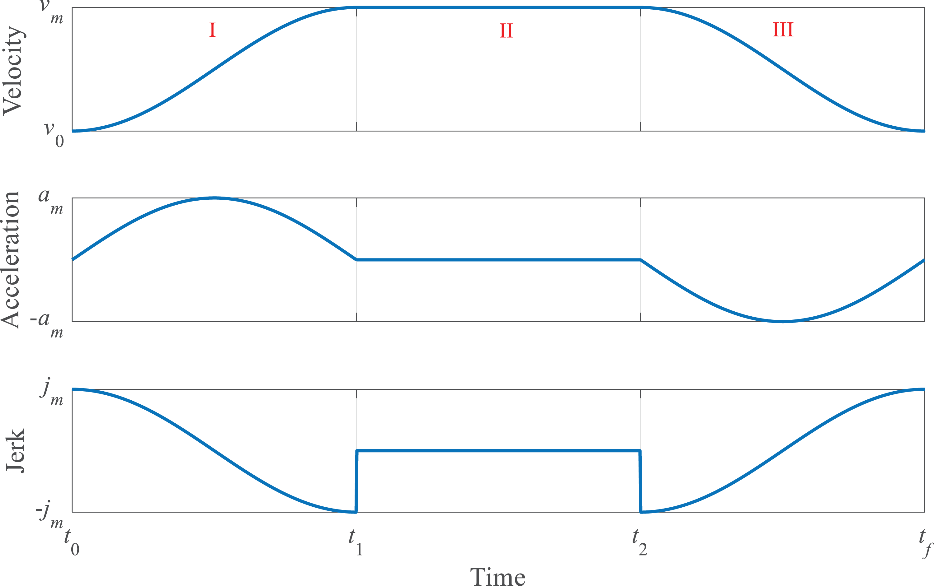
A sine curve.

Optimal S-curves and sine curves

For application considerations, the curve of motion profiles might be restricted by the hardware’s motion limits, such as maximum velocities, accelerations, and jerks. Thus, optimization approaches can be applied to determine the parameters of motion files. Consider that there are n_s piece functions of time to form a motion profile, and then an optimization problem is formulated to minimize the final time t_f as

\begin{matrix} min & J_{2} = t_{f} \end{matrix}

subject to

s^{(1)} (0) = s_{0}, {\dot{s}}^{(1)} (0) = v_{0}, {\ddot{s}}^{(1)} (0) = a_{0}

s^{(n)} (t_{f}) = s_{f}, {\dot{s}}^{(n)} (t_{f}) = v_{f}, {\ddot{s}}^{(n)} (t_{f}) = a_{f}

s^{(i)} (t_{i}) = s^{(i + 1)} (t_{i}), {\dot{s}}^{(i)} (t_{i}) = {\dot{s}}^{(i + 1)} (t_{i}), {\ddot{s}}^{(i)} (t_{i}) = {\ddot{s}}^{(i + 1)} (t_{i}), i = 1, 2, \dots, n_{s} - 1

0 < t_{1} < t_{2} < \dots < t_{n_{s} - 1} < t_{f}

max (| \dot{s} |) \leq v_{m}, max (| \ddot{s} |) \leq a_{m}, max (| \overset{⃛}{s} |) \leq j_{m}

where v_m , a_m , and j_m are the maximum velocity, acceleration, and jerk, respectively; equations (16) and (17) are the boundary conditions, where s ₀, v ₀, and a ₀ are, respectively, the initial position, velocity, and acceleration; s_f , v_f , and a_f are, respectively, the final position, velocity, and acceleration; equation (18) represents the continuities of position, velocity, and acceleration at the connecting points for two successive piecewise functions; equation (19) ensures that t_i is arranged in an ascending series; and equation (20) restricts the maximum velocities, accelerations, and jerks. Thus, the optimization problem can be solved by any optimization algorithms.

Optimal cubic curves

Alternatively, an optimal cubic curve consisting of multiple piece cubic polynomials is proposed to express a motion profile. Since the highest polynomial degree of the S-curve is 3, the proposed optimal cubic curve is a generalized formulation for S-curves. To illustrate the formulations of the curve, a curve is considered to be divided into n_s segments, and each segment is expressed to be a cubic polynomial as

s^{(i)} (t) = a_{0}^{(i)} + a_{1}^{(i)} t + a_{2}^{(i)} t^{2} + a_{3}^{(i)} t^{3}

where the superscript i represents the segment number; $a_{j}^{(i)}$ are the polynomial coefficients. Note that the number of segments n_s will be determined later, and the final time t_f is unknown. Similar to any motion profiles, the continuities of position, velocity, and acceleration should be satisfied between two successive segments, so there are $3 (n_{s} + 1)$ continuity equations, and the number of unknowns is $5 n_{s}$ , which is the sum of the numbers of polynomial coefficients and connecting points $t_{i} (i = 1, 2, \dots, n_{s} - 1)$ as well as t_f . It is worth to note that if an optimization problem is formed, the number of unknowns should be greater than or equal to the number of the equations, which leads to $n_{s} \geq 2$ . Therefore, a multisegment cubic curve with a minimum number of segments and minimum time can be obtained by determining the polynomial coefficients $a_{j}^{(i)} (i = 1, 2, \dots, n - 1 and j = 0, 1, 2, 3)$ , the time $t_{i} (i = 1, 2, \dots, n_{s} - 1)$ of the connecting points, the final time t_f , and the number of segments n_s through formulating a multiobjective optimization problem as

\begin{matrix} min_{a_{j}^{(i)}, t_{i}, t_{f}, n_{s}} & J = (t_{f}, n_{s}) \end{matrix}

subject to the constraints same as equations (16) to (20) and an additional constraint

n_{s} \geq 2 (n_{s} is an integer)

Figure 3 shows a three-segment cubic curve, where the Roman numerals refer to the segment numbers.

Figure 3.

A three-segment cubic curve.

Trajectory solver based on a path and a motion profile

The length of a parametric for a two-dimensional curve is given as

s (u) = \int_{0}^{u} \sqrt{{(\frac{d x}{d u})}^{2} + {(\frac{d y}{d u})}^{2}} d u

Taking the time derivative and applying Leibnitz rule lead to

\dot{s} (t) = \sqrt{{(\frac{d x}{d u})}^{2} + {(\frac{d y}{d u})}^{2}} \frac{d u}{d t}

Since the motion profile $\dot{s} (t)$ is obtained through those presented in “S-curves,” “Sine curves,” “Optimal S-curves and sine curves,” and “Optimal cubic curves” sections, equation (25) can be rewritten as

\dot{u} = \frac{\dot{s} (t)}{\sqrt{{(\frac{d x}{d u})}^{2} + {(\frac{d y}{d u})}^{2}}}

Note that equation (26) is a first-order nonlinear ordinary differential equation with the initial condition $u (0) = 0$ , and the numerator and the denominator of the right-hand side are functions of time and parameter u, respectively. Thus, equation (26) can be solved by using numerical methods.

Case study: Optimal trajectory planning of a dispensing robot

This section will investigate a case study, which is the trajectory planning for a dispensing robot. The robot will execute a dispensing motion for a 3.5-in hard drive, as shown in Figure 4(a). Besides, Figure 4(b) shows 44 measured control points surrounding the hard drive, and one will plan a path based on the 44 points. The optimal trajectory planning is a dual optimization procedure by optimizing the path and the motion profile presented in “Path planning based on parametric curves” and “Trajectory planning based on parametric curves” sections, respectively, and the design flowchart is shown in Figure 5.

Figure 4.

(a) A 3.5-in hard drive and (b) 44 control points around the hard drive.

Figure 5.

A flowchart of the dual optimization trajectory planning.

Optimal path planning

In this subsection, one will start the path planning by employing rational B-spline and then perform the path optimization to obtain a smoother path. The procedure of the path planning is illustrated as follows in detail.

One will apply a uniform rational B-spline with constant weighting values, where the order is 4 (the polynomial degree is 3), and the curve is shown in Figure 6(a). It is noted that the curve does not pass through all control points.

Figure 6.

Rational B-spline curves: (a) control points and virtual knots; (b) a uniform rational B-spline curve and an interpolation curve; (c) NURBS; and (d) optimal rational B-spline curves. NURBS: nonuniform rational B-spline curve.

Since the dispensing robot should pass through all control points, one applies the virtual-knot interpolation presented in “Virtual-knot interpolations” section, where the interpolation is based on the rational B-spline, and Figure 6(b) shows the interpolation curve. Besides, it is compared with the rational B-spline curve. It is obvious to see that the curve passes through all control points, but there is a cusp at the coordinates (4.6 and 13.5 cm), which are both the starting and the end points.

To smooth the cusp at the coordinates (4.6 and 13.5 cm), an NURBS is applied, and the differences of two successive knot values at the first and last few knots are increased to reduce the cusp. Thus, a knot vector consisting all knot values is defined as

\begin{matrix} u = [\begin{array}{l} 0 & 0 & 0 & 0 & 6 & 17 & 18 & 19 & 20 & \dots \end{array} \\ \begin{array}{l} \dots & 21 & 22 & 23 & 24 & 35 & 41 & 41 & 41 & 41 \end{array}] \end{matrix}

where 30 knot values between 20 and 21 form an arithmetic sequence. Based on the knot vector, an NURBS curve is shown in Figure 6(c), which includes two curves without pass through the control points and based on the virtual knots. It is obvious to see that the cusp has been greatly reduced.

Although the cusp has been reduced, the slope difference at the cusp is still greater than those at other control points. Thus, an optimization approach presented in “Optimal rational B-spline curves” section will be applied to minimize the slope differences at the cusp and the control points and the curve length. To simplify the optimization problem, the knot vector based on equation (27) is modified as

\begin{matrix} u = [\begin{array}{l} 0 & 0 & 0 & 0 & c & 17 & 18 & 19 & 20 & \dots \end{array} \\ \begin{array}{l} \dots & 21 & 22 & 23 & 24 & (41 - c) & 41 & 41 & 41 & 41 \end{array}] \end{matrix}

where c is the fifth knot value which will determine the optimization procedure, and the fifth last is modified as $(41 - c)$ due to the symmetry of the knot vector. Therefore, the optimization problem is expressed as

\begin{matrix} min_{c} & J \end{matrix} = w_{1} \frac{1}{n} {\sum_{i = 2}^{n + 1} ({\frac{d y}{d x}|}_{P_{i}} - {\frac{d y}{d x}|}_{P_{i - 1}})}^{2} + w_{2} {({\frac{d y}{d x}|}_{P_{n + 1}} - {\frac{d y}{d x}|}_{P_{1}})}^{2} + w_{3} \int_{u_{0}}^{u_{f}} \sqrt{{(\frac{d x}{d u})}^{2} + {(\frac{d y}{d u})}^{2}} d u

in which the weighting values w ₁, w ₂, and w ₃ are considered to be 0.0284, 0.0275, and 0.944, respectively, due to different value scales of the three terms. Based on the optimization problem, Figure 6(d) shows an optimal rational B-spline curve.

Optimal motion profile planning

This subsection presents the motion profile planning based on the optimization formulation shown in “Optimal S-curves and sine curves” and “Optimal cubic curves” sections, and the path is the optimal rational B-spline curve, as shown in Figure 6(d). For optimal S-curves, both five and seven segments are applied. For optimal cubic polynomials, since a multiobjective optimization leads to multiple solutions, both three and four segments are obtained. Due to the maximum velocity, acceleration, and jerk limited by the experimental robot, they should be restricted as

v_{max} \leq 3 (cm/s), a_{max} \leq 60 ({cm/s}^{2}), j_{max} \leq 1500 ({cm/s}^{3})

Thus, the results are listed in Table 1 by solving the minimum-time optimization problems. The results show that the optimal seven-segment S-curve provides the shortest motion time. To further examine the results, Table 2 lists some comparisons based on several specification indices, where $Δ t_{acc}$ , $Δ t_{con}$ , and $Δ t_{dec}$ represent the time periods of acceleration, constant or nearly constant speed, and deceleration, respectively. For maximum velocities, accelerations, and jerks, only the optimal five-segment S-curve does not reach the maximum velocity; only the optimal S-curves reach the maximum acceleration; the curves reach the maximum jerk except for the optimal cubic polynomials. In all curves, only the optimal seven-segment S-curve reaches the maximum velocity, acceleration, and jerk, so the curve has the shortest motion time. In general, each motion profile can be divided into three parts, increasing velocities, intermediate periods, and decreasing velocities, and the intermediate period is the longest time in each motion profile, which executes the majority of the entire motions. Besides, it is noted that the intermediate periods refer to constant velocities for the S-curve and the sine curve, which can shorten the motion time. However, since the optimal five-segment S-curve does not reach the maximum velocity, the motion time becomes longer. Furthermore, the proposed optimal cubic polynomials are not the best motion profiles in this subsection, because the curves are obtained through a multiobjective optimization procedure, which compromises the minimum time and the minimum number of segments.

Table 1.

Time of connecting points for minimum-time motion profiles.

t_i (s)	S-curves		Sine curve	Cubic polynomials
t_i (s)	Five segments	Seven segments	Three segments	Three segments	Four segments
t ₀	0	0	0	0	0
t ₁	0.0400	0.0400	0.0993	0.0010	0.9886
t ₂	0.0800	0.0500	13.0550	19.5826	0.2808
t ₃	16.3188	0.0900	—	—	17.5275
t ₄	16.3588	13.0550	—	—	—
t ₅	—	13.0950	—	—	—
t ₆	—	13.1050	—	—	—
t_f	16.3988	13.1450	13.1453	19.5836	17.5342

Table 2.

Comparisons of minimum-time motion profiles.

Specifications			S-curves		Sine curve	Cubic polynomials
Indices	Values	Units	Five segments	Seven segments	Three segments	Three segments	Four segments
$v_{max}$	3	cm/s	2.4	3	3	3	3
$a_{max}$	60	cm/s²	60	60	48	0.6	16
$j_{max}$	1500	cm/s³	1500	1500	1500	600	182
t_f	—	s	16.3988	13.1450	13.1453	19.5836	17.5342
$Δ t_{acc}$	—	s	0.0800	0.0900	0.0993	0.0010	0.2808
$Δ t_{con}$	—	s	16.2388	12.9650	12.9557	19.5816	17.2467
$Δ t_{dec}$	—	s	0.0800	0.0900	0.0903	0.0010	0.0067

Combinations of the optimal path and the optimal motion profile

Based on the results of “Optimal path planning” and “Optimal motion profile planning” sections, the optimal path is based on the nonuniform ration B-spline (NURBS), and the optimal motion profile is based on the seven-segment S-curve. By solving equation (26) through imposing the optimal path and the optimal motion profile, the parameter u of the parametric curve can be obtained, as shown in Figure 7(a), and the trajectories of x- and y-coordinates can be further calculated, as shown in Figure 7(b) and 7(c), respectively, which can be applied to a dispensing robot to accomplish a dispensing motion for the 3.5-in hard drive.

Figure 7.

Optimal trajectories of (a) parameter u; (b) x-coordinate; and (c) y-coordinate.

Experimental results

In this study, an experimental Delta robot is used to simulate the motion of a dispensing robot by tracking the planned trajectory obtained in “Combinations of the optimal path and the optimal motion profile” section, but the robot does not have a dispensing head. The Delta robot is a spatial parallel manipulator, as shown in Figure 8. There are three brushed DC motors mounted on a fixed plane, and each motor drives a kinematic chain consisting of two links, where the connecting joint of the two links is a spherical joint. Besides, three kinematic chains connect a moving platform by spherical joints, and the moving platform is called an end effector, which is dominated by the motions of the three motors. Therefore, the Delta robot has three degrees of freedom, which are three translating motions in three-dimensional space, and a gripper is usually mounted on the end effector to fulfill a pick-and-place task. For a dispensing robot, a dispensing head can be mounted on the end effector, and it will track a planned trajectory to execute a predefined motion.

Figure 8.

An experimental Delta robot.

To operate the robot, the planned trajectory needs to be transformed the motions of the three motors through the inverse kinematics, which can be obtained by solving three nonlinear algebraic equations, and then the calculated motions of the motors will be executed by performing the feedback control of the motors. In the experiments, the motor control is achieved by using a real-time embedded system CompactRIO (shown in Figure 9), manufactured by National Instruments, Inc., and three proportional–integral–derivative (PID) controllers are designed and implemented in the system, where the encoder mounted on the motors and the encoder signals are delivered to the system in order to fulfill the feedback control of motors. The PID controller parameters are obtained by using the function pidTuner of the software MATLAB, where the motor model is obtained through system identification by using the software MATLAB, too.

Figure 9.

An embedded system CompactRio.

Figure 10 shows the command signals, simulation, and experimental results of the active angles as functions of time. The simulation results and the command signals are quite consistent, and the experimental results are stair functions of time due to the limited resolutions of the encoders, which are 0.367°. Figure 11 shows the command, simulation, and experimental results of the position of the end effector as functions of time. The simulation results and the command signals are also quite consistent, and the experimental results show little variations due to the experimental errors. Figure 12 shows the virtual control points and the trajectory of the command signals, the simulation, and experimental results on the x–y plane. As expected, the command trajectory passes through all virtual control points. The simulation results are consistent with the command trajectory, but the experimental results show little variations from the desired trajectory. To examine the errors, the errors are defined as the differences between the command signals and the simulation as well as experimental results, and Table 3 presents the root mean square errors. For the active angles, the simulation errors are less than 0.01°, and the experimental errors are around 0.1°. For the positions of the end effector, the simulation errors of the x-and y-coordinates are around 0.1 mm, and the experimental errors are around 1 mm. For the trajectory error, the simulation error is 0.1427 mm, and the experimental error is 1.3914 mm. The simulation errors come from the motor dynamics and the controller performance. The experimental errors are caused by not only the dynamics of the robot and the controller performance but also the hardware inaccuracy, including the manufacturing error of the robot, the resolutions of the encoders, the signal transmission delays, the capability of the controller, and so on. This case study simply demonstrates the validity of the proposed optimal trajectory planning, which can be applied to a dispensing robot.

Figure 10.

Command, experimental, and simulation rotating angles of the motors as functions of time: (a) θ ₁; (b) θ ₂; and (c) θ _3.

Figure 11.

Experimental and simulation positions of the end effector as functions of time: (a) x-coordinate; (b) y-coordinate; and (c) z-coordinate

Figure 12.

Trajectories of the command, simulation, experiment results and the control points of the end effectors on the x–y plane.

Table 3.

RMS errors of the experimental and simulation results.

Symbols	θ ₁	θ ₂	θ ₃	x	y	z	e _p
Units	°	°	°	mm	mm	mm	mm
Simulation	0.0634	0.0705	0.0618	0.1160	0.0729	0.0399	0.1427
Experiment	0.1030	0.1124	0.1080	0.9277	1.0370	0.0376	1.3914

RMS: root mean square; e _p: trajectory error.

Conclusions

This article presents the optimal trajectory planning and tracking control of a Delta robot, which is used to simulate the motion of a dispensing robot. B-spline curves are commonly used to plan a path, but they do not pass through control points. To solve this problem, a virtual-knot based interpolation scheme is proposed, which can pass through all control points by employing an inverse procedure. To design a smoother path, an optimization formulation is proposed to minimize the slope variations of the path, where the knot vector and the weighting values of the rational B-spline can be obtained by solving the optimization problem. Regarding the trajectory planning, a multisegment piecewise cubic polynomial is proposed, which is a generalized S-curve, where the curve parameters including the polynomial coefficients and the number of segments are obtained by solving a multiobjective optimization problem. Besides, another optimization formulation is proposed to minimize the motion time, where the parameters of motion profiles can be obtained by solving this optimization problem. Furthermore, the planned trajectory is applied to an experimental Delta robot so as to simulate the dispensing motion, and the experimental results show that the trajectory error is less than 2 mm based on the hardware specifications of the experimental Delta robot. As a matter of fact, the proposed approach can be applied to any types of robots and machine tools, which are used for machining, such as turning, drilling, and milling, in practical applications.

Footnotes

Declaration of conflicting interests

The author(s) declared no potential conflicts of interest with respect to the research,authorship,and/or publication of this article.

Funding

The author(s) disclosed receipt of the following financial support for the research,authorship,and/or publication of this article: This work was supported in part by the Ministry of Science and Technology [Grant MOST 107-2221-E-011-135].

ORCID iD

Yong-Lin Kuo

References

González

Pérez

Milanés

, et al. A review of motion planning techniques for automated vehicles. IEEE Trans Intell Transp Syst 2015; 17(4): 1135–1145.

Jahanpour

Motallebi

Porghoveh

. A novel trajectory planning scheme for parallel machining robots enhanced with NURBS curves. J Intell Robot Syst 2016; 82(2): 257–275.

Choi

Kim

Hwang

, et al. Dual-arm robot motion planning for collision avoidance using B-spline curve. Int J Precis Eng Man 2017; 18(6): 835–843.

Cheng

Wang

, et al. Time-optimal trajectory planning for delta robot based on quintic Pythagorean-hodograph curves. IEEE Access 2018; 6: 28530–28539.

Chettibi

. Smooth point-to-point trajectory planning for robot manipulators by using radial basis functions. Robotica 2019; 37(3): 539–559.

Meckl

Arestides

. Optimized s-curve motion profiles for minimum residual vibration. In: Proceedings of the 1998 American control conference (eds Chow

Heck

), Vol. 5, Philadelphia, Pennsylvania, USA, 24–26 June 1998, pp. 2627–2631. IEEE.

Nguyen

Chen

. On algorithms for planning s-curve motion profiles. Int J Adv Robot Syst 2008 5(1): 99–106.

Yang

Jiang

. Fast trajectory planning for VGT manipulator via convex optimization. Int J Adv Robot Syst 2015; 12(9): 136.

Zhang

Wang

Zhou

. Trajectory planning of 7-DOF space manipulator for minimizing base disturbance. Int J Adv Robot Syst 2016; 13(2): 44.

10.

Huang

, et al. Optimal time-jerk trajectory planning for industrial robots. Mech Mach Theory 2018; 121: 530–544.

11.

Chen

Yang

ECY

. Near time-optimal s-curve velocity planning for multiple line segments under axis constraints. IEEE Trans Aerosp Electron 2018; 65(12): 9582–9592.

12.

Zhai

, et al. A novel non-collision trajectory planning algorithm based on velocity potential field for robotic manipulator. Int J Adv Robot Syst 2018; 15(4):1–13.

13.

Consolini

Locatelli

Minari

, et al. Optimal time-complexity speed planning for robot manipulators. IEEE Trans Robot 2019; 35(3): 790–797.

14.

Fang

Liu

, et al. Smooth and time-optimal S-curve trajectory planning for automated robots and machines. Mech Mach Theory 2019; 137: 127–153.

15.

Wen

, et al. Q-learning trajectory planning based on Takagi-Sugeno fuzzy parallel distributed compensation structure of humanoid manipulator. Int J Adv Robot Syst 2019; 16(1): 1–17.

16.

Zajačko

Gál

Ságová

, et al. Application of artificial intelligence principles in mechanical engineering. MATEC Web of Conferences 2018: 244: 01027.

17.

Pivarčiová

Božek

Turygin

, et al. Analysis of control and correction options of mobile robot trajectory by an inertial navigation system. Int J Adv Robot Syst 2018: 15(1): 1–15.

18.

Bozek

Pokorný

Svetlík

, et al. The calculations of Jordan curves trajectory of the robot movement. Int J Adv Robot Syst 2016: 13(5): 1–7.

19.

Trnka

Božek

. Optimal motion planning of spot welding robot applications. Appl Mech Mater 2013: 248: 589–593.

20.

Tlach

Císar

Kuric

, et al. Determination of the industrial robot positioning performance. MATEC Web Conf 2017: 13: 01004.

21.

Ata

. Optimal trajectory planning of manipulators: a review. J Eng Sci Technol 2007; 2(1): 32–54.

22.

Jeevamalar

Ramabalan

. Optimal trajectory planning for autonomous robots - a review. In: IEEE international conference on advances in engineering, science and management (eds Pillay

CGS

Paramesvaran

), Nagapattinam, Tamil Nadu, India, 30–31 March 2012, pp. 269–275. IEEE.

23.

Gao

Zhang

. A review of the space trajectory planning of redundant manipulator. J Mech Eng 2016; 10: 176–180.

24.

Mohanan

Salgoankar

. A survey of robotic motion planning in dynamic environments. Robot Auton Syst 2018; 100: 171–185.

25.

Shang

. Research of trajectory planning for articulated industrial robot: a review. Comput Eng Appl 2018; 54(5): 36–50.

26.

Yang

Pan

Wan

. Survey of optimal motion planning. IET Cyber-Systems Robot 2019; 1(1): 13–19.

27.

Ahlberg

Nilson

Walsh

. The Theory of Splines and Their Applications 1st ed. Cambridge: Academic Press, 1967.

28.

Bézier

. How Renault uses numerical control for car body design and tooling. In: Automotive Engineering Congress and Exposition Detroit, MI, 1968, SAE paper 680010.

29.

Gordon

Riesenfeld

. Bernstein-Bézier methods for the computer aided design of free-form curves and surfaces. J ACM 1974; 21: 293–310.

30.

Schoenberg

. Contributions to the problem of approximation of equidistant data by analytic functions. Q Appl Math 1946; 4(2): 112–141.

31.

Cox

. The numerical evaluation of B-splines. J Appl Math 1972; 10(2): 134–149.

32.

de Boor

. On calculation with B-splines. J Approx Theory 1972; 6:50–62.

33.

Versprille

. Computer-aided Design Applications of the Rational B-spline Approximation Form. Ph.D. dissertation, Syracuse University, 1975.

34.

Smith

Wellington

. Initial graphics exchange specification (IGES), Version 3.0, National Bureau of Standard Publications, No. PB86-199759, Gaithersburg, MD, 1986.

35.

Chen

. Genetic algorithm-based S-curve acceleration and deceleration for five-axis machine tools. Int J Adv Manuf Tech 2016; 87(1-4): 219–232.

36.

Liu

Chen

. Combined S-curve feedrate profiling and input shaping for glass substrate transfer robot vibration suppression. Ind Robot 2018; 45(4): 549–560.

37.

Gong

Wang

Zhao

, et al. Bionic quadruped robot dynamic gait control strategy based on twenty degrees of freedom. IEEE/CAA J Autom Sin 2017; 5(1): 382–388.

38.

Ariizumi

Takahashi

Tanaka

, et al. Head-trajectory-tracking control of a snake robot and its robustness under actuator failure. IEEE T Cont Syst Tech 2018; 99: 1–9.

39.

Xue

Dong

Yan

. Sliding mode variable structure based path following control of agricultural robots with differential drive. IFAC-PapersOnLine 2018; 51(17): 455–459.