Sage Journals: Discover world-class research

Abstract

In understanding Big Data, people are interested to obtain the trend and dynamics of a given set of temporal data, which in turn can be used to predict possible futures. This paper examines a time series analysis method and an ordinary differential equation approach in modeling the price movements of petroleum price and of three different bank stock prices over a time frame of three years. Computational tests consist of a range of data fitting models in order to understand the advantages and disadvantages of these two approaches. A modified ordinary differential equation model, with different forms of polynomials and periodic functions, is proposed. Numerical tests demonstrated the advantage of the modified ordinary differential equation approach. Computational properties of the modified ordinary differential equation are studied.

Keywords

Time series analysis autoregressive integrated moving average ordinary differential equation mean absolute percentage error

Introduction

Observing the trend and forecasting the future are always required in all kinds of market. In understanding Big Data, people are more interested to obtain the trend and dynamics of a given set of temporal data, which in turn can be used to predict possible futures.

Classic statistical methods are usually used to perform the task, such as regression analysis, cluster analysis, and so on. As a branch of statistics, time series analysis (TSA) is very popular for modeling temporal data.¹ Great efforts have been put in the application of TSA in the temporal market analysis. In 1970, Box and Jenkins proposed the autoregressive integrated moving average (ARIMA) model.² In order to handle time-varying property of variance, Engle derived autoregressive conditional heteroscedasticity (ARCH) model.³ Next, Bollerslev (1986), Glosten et al. (1991), and Nelson (1991) derived generalized ARCH (GARCH) model, threshold ARCH (TARCH) model, and exponential ARCH (EARCH) model, respectively.

One of the disadvantages of these statistical methods is that large amount of market data is required. In such cases, numerical methods, i.e. ordinary differential equations (ODE),⁴ partial differential equations (PDE), or stochastic differential equations (SDE), would be taken into account.

This paper examines a modified ODE approach and compares it with TSA in modeling the price movements of petroleum price and of three different bank stock prices over a time frame of three years. The market data were obtained from the official web page.⁵ Computational tests consist of a range of data fitting models in order to understand the advantages and disadvantages of these two approaches. Then, a modified ODE model, with different forms of polynomials and periodic functions, is proposed. Numerical tests demonstrate the advantages of such modification. Computational properties of the modified ODE are studied.

The rest of this article is organized as follows. In the upcoming section, ARIMA model and an ODE method are introduced and then results of them are compared. Subsequently, the modification of the ODE model is presented and the empirical analysis is shown. Finally, the article is concluded in the last section.

The ARIMA and the existing ODE models

Fundamental methods

Time series analysis comprises methods for analyzing temporal data. Models for time series data contain many forms representing different stochastic processes. In statistics and econometrics, and in particular in TSA, the autoregressive integrated moving average (ARIMA) models are often applied in some cases where data show evidence of nonstationary. Wan and Wen⁶ found that ARCH model did not always show better compared to ARIMA model. For simplicity, attention was only given to ARIMA model in this section.

ARIMA models are generally denoted by ARIMA $(p, d, q)$ where parameters $p, d,$ and $q$ are nonnegative integers, $p$ is the order of the autoregressive model, $d$ is the degree of differencing, and $q$ is the order of the moving average model.⁷

Given the time series of data $y_{t}$ where $t$ is an integer index and $y_{t}$ is a real number, then an ARIMA $(p, d, q)$ model is given by $(1 - \sum_{i = 1}^{p} φ_{i} B^{i}) Δ^{d} y_{t} = (1 - \sum_{i = 1}^{q} θ_{i} B^{i}) ε_{t}$ (1)where $B$ is the lag operator such that $B^{k} y_{t} = y_{t - k}, k = 0, 1, 2, \dots$

And the symbol $Δ$ is the differencing operator such that $Δ^{d} y_{t} = {(1 - B)}^{d} y_{t}, d = 0, 1, 2, \dots$

$φ_{i}$ are the parameters of the autoregressive part, $θ_{i}$ are the parameters of the moving average part, and $ε_{t}$ are white noise error terms.

Case $d = 0$ corresponds to the ARMA $(p, q)$ model. What’s worth mentioning is that the ARMA $(p, q)$ models are used for the stationary data. If data is nonstationary, one should try ARIMA $(p, d, q)$ models. Finally, one could determine the best model according to the Akaike information criterion (AIC) or the Bayesian information criterion (BIC).

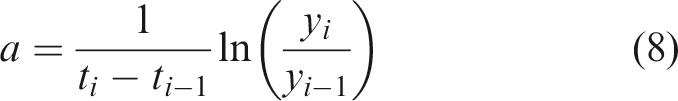
Next, considering the Cauchy initial value problem $y^{'} = a y, y (t_{0}) = y_{0}$ (2)

One can solve equation (2) by means of numerical integration or obtain an analytic solution if $a$ is given. It is also possible to calibrate $a$ at different time intervals.

One approach for solving equation (2) is given by Lascsáková.⁸ The particular solution of problem (2) is $y = y_{0} e^{a (t - t_{0})}$

Substituting the point $(t_{1}, y_{1})$ to this particular solution, we have $y_{1} = y_{0} e^{a (t_{1} - t_{0})}$ (3)

From equation (3), $a$ is obtained as follows $a = \frac{1}{t_{1} - t_{0}} \ln (\frac{y_{1}}{y_{0}})$ (4)

At the next time $t_{2}$ , one has $y_{2} = y_{1} e^{a (t_{2} - t_{1})}$ (5)

From equation (5), $a$ is obtained again $a = \frac{1}{t_{2} - t_{1}} \ln (\frac{y_{2}}{y_{1}})$ (6)

Generalizing the previous principle, one can get the solution of problem (2) in the following form $y_{i + 1} = y_{i} e^{a (t_{i + 1} - t_{i})}$ (7)

Here, $a = \frac{1}{t_{i} - t_{i - 1}} \ln (\frac{y_{i}}{y_{i - 1}})$ (8)

Comparison of the TSA and the existing ODE model

This section compares the time-domain TSA method given in equation (1) and the ODE approach given in equation (2) in modeling the price movements of petroleum price and of two bank stock prices over a time frame of three years.

For the observed data $(t_{0,} y_{0}), (t_{1,} y_{1}), (t_{2,} y_{2}), \dots, (t_{n,} y_{n})$ of a time series of data $y_{t}$ , the absolute percentage error (APE) and mean of APE (MAPE) are chosen applied as the criterion to evaluate the models in this paper. They are defined as $A P E_{i} = \frac{| {\hat{y}}_{i} - y_{i} |}{y_{i}}$ $M A P E = \frac{1}{n} \sum_{i = 1}^{n} A P E_{i}$

Let ${\hat{y}}_{i}$ denote the approximated value at time (day/month/year) $t_{i}$ , $y_{i}$ denotes the observed value at time (day/month/year) $t_{i}$ . Although MAPE is less often used than the mean square error (MSE) and the mean absolute error (MAE), it is a more natural error measure, and has several advantages.⁹

For petroleum data in 2013, an appropriate model is ARIMA(0, 1, 13) $x_{t} = x_{t - 1} + ε_{t} - 0.1338 ε_{t - 5} - 0.1226 ε_{t - 13}$

The calculated results are shown in Table 1. The table indicates that all the APEs of TSA are less than 5%. There are 249 APEs of ODE and only one APE of ODE is not less than 5% but less than 7.5%. It seems that there is almost no difference between these two approaches in this sense. But, the MAPE of TSA is less than that of ODE. It is well known that APE and MAPE are the smaller the better. As a consequence, the TSA method is preferred in the market.

Table 1.

Comparing ODE and TSA of petroleum price (2013).

APE	ODE	TSA
[0, 5%)	249	250
[5%, 7.5%)	1	0
[7.5%, 10%)	0	0
[10%, 1)	0	0
MAPE	1.2597%	0.8817%

APE: absolute percentage error; ODE: ordinary differential equation; TSA: time series analysis.

For petroleum data in 2014, an appropriate model is ARIMA(6, 1, 0) $\begin{matrix} x_{t} = - 0.1662 + 0.8299 x_{t - 1} + 0.1701 x_{t - 2} + 0.1727 x_{t - 6} \\ - 0.1727 x_{t - 7} + ε_{t} \end{matrix}$

For petroleum data in 2015, an appropriate model is ARIMA(1, 1, 0) $x_{t} = 0.8695 x_{t - 1} + 0.1305 x_{t - 2} + ε_{t}$

The results of comparing ODE and TSA of petroleum price (2014, 2015) are shown in Tables 2 and 3.

Table 2.

Comparing ODE and TSA of petroleum price (2014).

APE	ODE	TSA
[0, 5%)	235	248
[5%, 7.5%)	9	1
[7.5%, 10%)	4	0
[10%, 1)	2	1
MAPE	1.7445%	1.0670%

APE: absolute percentage error; ODE: ordinary differential equation; TSA: time series analysis.

Table 3.

Comparing ODE and TSA of petroleum price (2015).

APE	ODE	TSA
[0, 5%)	198	227
[5%, 7.5%)	30	18
[7.5%, 10%)	15	5
[10%,1)	7	0
MAPE	3.4100%	2.2922%

APE: absolute percentage error; ODE: ordinary differential equation; TSA: time series analysis.

Similarly, this paper also worked on the share values of two banks over a period of about 750 days. The results are obtained in Table 4.

Table 4.

Comparing ODE and TSA of bank share values.

APE	Barclays bank		Lloyds bank
APE	ODE	TSA	ODE	TSA
[0, 5%)	623	694	626	706
[5%, 7.5%)	90	54	82	39
[7.5%, 10%)	39	14	41	19
[10%, 1)	20	10	22	8

APE: absolute percentage error; ODE: ordinary differential equation; TSA: time series analysis.

From the above examples, TSA seems to show better results compared to ODE. However, it is possible to modify the form of the derivative given in equation (2).

Modification of the ODE model

There are different ways of modifying the ODE model given in equation (2). For example, the form of the derivative given in equation (2) may be changed. This section introduces several alternatives in such modification.

If the data $y_{t}$ is not an exponential function of time variable $t$ , equation (2) may be modified. Equation (8), which in fact defined the parameter $a$ as a piecewise function, may also be modified. Hence, the modification consists of the derivative itself and the parameter $a$ . After modification, problem (2) can be transformed into $y^{'} = f (y), y (t_{0}) = y_{0}$ (9)or $y^{'} = f (t) y, y (t_{0}) = y_{0}$ (10)

Several different forms of $f (.)$ as listed in Table 5 have been tested.

Table 5.

Possible forms of $f (x)$ .

$α \sin x + β$	$α e^{x} + β$
$α x + β$	$\frac{α x}{β + x}$
$α x^{2} + β x + γ$	$α \cdot 2^{- x / β}$
$α \ln x + β$	$α β^{x}$
$α \sin x + β x + γ$	$α + β γ^{x}$
$α \sin x + β \ln x + γ$	$e^{α + β γ^{x}}$
$α \ln x + β x + γ$	$\frac{1}{α + β γ^{x}}$
$α \sin x + β x + γ \ln x + δ$	$α e^{β x} + γ$
…	…

Problems (9) and (10) are actually separable differential equations. A general form, which leads to a nonseparable differential equation, is given as below $y^{'} = a (t) y + s (y)$ (11)

It should be noted that $s (y)$ is itself a function of $y$ . The forms of $a (t)$ and $s (y)$ could be the primary functions, such as exponential function, trigonometric function, logarithmic function, and power function. Primary functions could be expanded to power series under special conditions. Furthermore, sometimes the data $y_{t}$ might be periodic. Henceforth, the derivative $y'$ might consist of a polynomial and a periodic function. A generalized model is given as below $y^{'} = g (t, y) = (\sum_{i = 0}^{M} a_{i} t^{i}) y + b_{0} + \sum_{j = 1}^{N} b_{j} sin (\frac{2 π j y}{θ} + c_{j})$ (12)

The unknown parameters $a_{0}, a_{1}, \dots, a_{M}, b_{0}, b_{1}, \dots, b_{N}, c_{1}, c_{2}, \dots, c_{N}, θ$ are estimated according to the approach of inverse problem.¹⁰ The numerical solution is obtained by fourth-order Runge–Kutta one-step method, which is the most widely known member of the Runge–Kutta family.¹¹ $y_{n + 1} = y_{n} + \frac{1}{6} h (k_{1} + 4 k_{2} + k_{3}),$ where $h = t_{n + 1} - t_{n},$ $k_{1} = g (t_{n}, y_{n}),$ $k_{2} = g (t_{n} + \frac{1}{2} h, y_{n} + \frac{1}{2} h k_{1}),$ $k_{3} = g (t_{n} + \frac{1}{2} h, y_{n} + \frac{1}{2} h k_{2}),$ $k_{4} = g (t_{n} + h, y_{n} + h k_{3})$

The bigger the values of $M$ or $N$ , the more will be the number of parameters to be estimated. Furthermore, the bigger the values of $M$ or $N$ , the more likely that the Jacobian matrix is singular. It should be noted that the bigger the values of $M$ or $N$ , the more difficult will be the computational work. From all these points of view, one would usually take $M$ or $N$ to be less than four.

Empirical analysis

Applying the above ODEs (9), (10), (11), and (12) to the petroleum data and three bank share prices, some improved results are obtained. In practice, one would prefer equation (12), which consists of a polynomial and a periodic function. The results are shown in Tables 6 to 11.

Table 6.

MAPE of petroleum (2013) according to equation (12).

MAPE		N
MAPE		1	2	3
M	0	0.89524%	0.88784%	0.88896%
	1	Singular	0.89059%	0.88722%
	2	Singular	Singular	Singular
	3	Singular	Singular	Singular

MAPE: mean absolute percentage error.

Table 7.

MAPE of petroleum (2014) according to equation (12).

MAPE		N
MAPE		1	2	3
M	0	1.08986%	1.11213%	1.10441%
	1	Singular	Singular	1.09418%
	2	Singular	Singular	Singular
	3	Singular	Singular	Singular

MAPE: mean absolute percentage error.

Table 8.

MAPE of petroleum (2015) according to equation (12).

APE		N
APE		1	2	3
M	0	2.27096%	2.26665%	2.30960%
	1	2.25025%	2.26416%	2.26109%
	2	Singular	Singular	Singular
	3	Singular	Singular	Singular

APE: absolute percentage error.

Table 9.

MAPE of Barclays bank according to equation (12).

APE		N
APE		1	2	3
M	0	2.23898%	Singular	Singular
	1	2.25212%	Singular	Singular
	2	Singular	Singular	Singular
	3	Singular	Singular	Singular

APE: absolute percentage error.

Table 10.

MAPE of Lloyds bank according to equation (12).

APE		N
APE		1	2	3
M	0	2.29275%	2.30361%	2.31223%
	1	2.29840%	2.29030%	2.31427%
	2	Singular	Singular	Singular
	3	Singular	Singular	Singular

APE: absolute percentage error.

Table 11.

MAPE of RBS bank according to equation (12).

APE		N
APE		1	2	3
M	0	2.21889%	2.21824%	2.21455%
	1	2.21350%	2.21267%	Singular
	2	Singular	Singular	Singular
	3	Singular	Singular	Singular

APE: absolute percentage error.

In the aforementioned tables, one could choose the best model with the smallest MAPE. For example, for petroleum data in 2013, the smallest MAPE occurs when $M = 1$ and $N = 3$ . For Barclays bank, the smallest MAPE occurs when $M = 0$ and $N = 1$ . The parameters are estimated according to the approach for inverse problem. Results are as shown in Table 12.

Table 12.

The estimated parameters.

Parameters	Petroleum			Bank
Parameters	2013	2014	2015	Barclays	Lloyds	RBS
$a_{0}$	−0.03031	0.01215	−0.02185	−0.00947	−0.00638	−0.00914
$a_{1}$	0.00001		−0.00004		−0.00001	−0.00002
$b_{0}$	2.90619	−1.30755	1.26420	2.36196	0.43602	4.88964
$b_{1}$	0.24353	−0.22307	0.16355	1.31137	−0.07560	0.82936
$θ$	0.49755	0.74135	0.46282	0.50023	0.49999	0.49879
$c_{1}$	−4.50499	398.30817	12.81797	1.56126	49.13539	−8.37850
$b_{2}$	−0.17368				0.18431	0.84405
$c_{2}$	−11.26577				1.52255	−5.84867
$b_{3}$	0.11570
$c_{3}$	−15.31979

The results of equations (2) and (12) can be compared. As can be seen in Table 13 the modified ODE given in equation (12) does improve the results with regard to MAPE.

Table 13.

MAPE compared with different $y'$ .

	Model given in equation (2)	Model given in equation (12)
Petroleum 2013	1.2597%	0.8872%
Petroleum 2014	1.7445%	1.0809%
Petroleum 2015	3.4100%	2.2471%
Barclays	3.2526%	2.2390%
Lloyds	3.1877%	2.2855%
RBS	3.0739%	2.2127%

Conclusions

In order to obtain the trend and forecast the future with higher accuracy, the idea of modifying the ODE model is proposed and the form as in equation (12) seems to be the best modification. Based on the obtained result, it can be stated that such modification provides good understanding of the trend and the dynamics of the price movement. This provides a good way forward in forecasting. Furthermore, on comparison with the statistical methods, numerical methods for ODEs show that fewer historical market data are required.

Finally, recalling the following problem, which involves a deterministic function $μ (t, y)$ $y^{'} = μ (t, y)$ (13)

This paper provides an insight on various forms of the right-hand side of problem (13). The authors anticipate that this work will lead to a systematic and an accessible way of forecasting the dynamic market, particularly some of the price movements in the financial market. The results are calculated with R.¹²

Footnotes

Declaration of conflicting interests

The author(s) declared no potential conflicts of interest with respect to the research,authorship,and/or publication of this article.

Funding

The author(s) received no financial support for the research,authorship,and/or publication of this article.

References

Tsay

RS.

Analysis of financial time series. 2nd ed. New York: John Wiley & Sons, 2005.

Engle

RF.

Autoregressive conditional heteroskedasticity with estimates of the variances of UK inflation. Econometrica 1982; 31: 987–1008.

Bolleslev

Generalized autoregressive conditional heteroskedasticity. J Econom 1986; 31: 307–327.

Gear

CW.

Numerical initial value problems in ordinary differential equations. Englewood Cliffs, NJ: Prentice-Hall, 1971.

http://www.eia.gov/dnav/pet/pet_pri_spt_s1_d.htm

Wan

J and

Wen

The comparison of ARIMA model and ARCH model application in Hong Kong stock price index prediction. J Appl Stat Manage 2001; 20: 1–4.

https://en.wikipedia.org/wiki/Autoregressive_integrated_moving_average

Lascsáková

The numerical model of forecasting aluminium prices by using two initial values. Studies of the University of Žilina, Mathematical Series, 2009, vol.23, pp. 85–92.

De Myttenaere

et al . Mean absolute percentage error for regression models. Neurocomputing 2016; 192: 38–48.

10.

Aster

et al . Parameter estimation and inverse problems. 2nd ed. Amsterdam: Elsevier, 2012.

11.

Delin

T and

Zheng

On a general formula of fourth order Runge-Kutta method. J Math Sci Math Educ 2012; 7: 1–10.

12.

Cryer

Chan

KS.

Time series analysis with applications in R. 2nd ed. New York: Springer-Verlag, 2008.