
Abstract

Introduction
Spices have traditionally been an expensive commodity. Consumers’ exposure to, and acceptance of, a larger diversity of culinary flavors has increased demand for spices of worldwide provenance, resulting in a more complex supply chain and increasing the business's vulnerability to adulteration.1,2 According to public opinion polls, food safety is one of the top consumer concerns.3,4 Although consumers are happy with their access to a variety of spice preferences, safety concerns exist among the general public, as well as regulatory authorities responsible for preserving and ensuring the safety and purity of spices. Recent reports 5 showed the presence of many adulterants in spices that are considered highly toxic to human health. Cowell et al. 6 reported widespread poisonous lead chromate (LC) contamination of turmeric (TU) powder sold in U.S. grocery stores with actual cases of lead poisoning in children across many U.S. states linked to the consumption of the contaminated products.
With more stakeholders in the spice supply chain and a larger danger of misrepresentation, effective authenticity testing and monitoring methods are required to deal with the growing challenges. In recent years, much effort has gone into developing vibrational spectroscopy fingerprint techniques for determining food quality and authenticity.7,8 In terms of analytical speed, cost, and environmental impact, vibrational spectroscopy-based techniques offer a viable and reliable alternative to traditional methods. Furthermore, these approaches rely on direct bulk analysis, which entails working directly on the food item with little or no sample preparation, as opposed to the extraction and concentration steps often used when using traditional testing methods. Fingerprint spectral matching to a large database is the most basic method for substance identification. This approach is very useful when working with pure compounds or with consistent ingredients. When working with randomly mixed materials, however, this strategy becomes less effective. As a result, the strength of infrared (IR) spectroscopy is derived from its combined use with chemometrics, which are primary linear-based models capable of extracting and summarizing underlying features in spectral data sets of both pure and mixed materials.9,10 With recent advances in data science, a variety of machine learning (ML) techniques for extracting information from multivariate data has been developed. Because ML and chemometrics perform similar tasks, their integration has created a larger pool of algorithms capable of linear and nonlinear feature extraction for improved classification and prediction problems. 10
Turmeric (TU) is made from the rhizomes of the tropical plant
Principal component analysis (PCA) and partial least squares (PLS) regression are most likely the two linear-based approaches most commonly employed to decrease dimensionality and extract features for data exploration, as well as subsequent classification and prediction analyses of food adulterants. In addition to being a novel nonlinear approach, the t-distributed stochastic neighbor embedding (t-SNE) method 14 has also been shown to be very versatile and well-suited for transforming high-dimensional data sets into low-dimensional plots, especially for data exploration tasks.15,16 As a popular artificial intelligence (AI) tool, t-SNE has found uses in a wide range of scientific disciplines, including medicine and bioinformatics, 17 and it could potentially be used in food safety investigations.
Feature reduction is a technique used to improve the computation efficiency and accuracy of multivariate data. When applied to spectral data, this means reducing the number of wavenumber variables by selecting the most important ones and excluding those that are redundant and have little explanatory value for analysis. The combinations of principal component-linear discriminant analysis (PC–LDA) and partial least-squares-discriminant analysis (PLS–DA) are examples of algorithms that combine feature extraction and classification tasks. Instead of the original data, these algorithms construct classification models based on chosen latent variables from PCA and PLS analysis. The usage of ensemble learning models, which combine the decisions of several models to enhance the final overall output, is another technique used to improve classification and prediction outcomes. Random forest (RF) is a common ensemble learning model based on decision trees that is noted for its performance. 18
Deep learning (DL), a branch of ML and AI, 19 has gained significant popularity in recent years. It is based on supervised algorithms called artificial neural networks (ANNs), which are computational models inspired by the structure of biological neural networks.20,21 ANNs have been introduced as a data-driven self-learning computing system for decades but were limited in use due to a lack of processing power and other factors such as limited data availability, computational efficiency, and difficulty in optimizing the network architecture and hyperparameters. However, with technological advancements, they have become a leading state-of-the-art algorithm. In recent years, DL applications have taken over numerous critical processes we depend on daily, including computer vision, speech recognition, internet search, fraud detection, email/spam filtering, financial risk modeling, medical diagnosis, self-driving vehicles, navigation, drug discovery, item identification, and more. 22
Convolutional neural network (CNN) is one of the most widely used and established DLs, particularly in the areas of computer vision. DL neural networks such as CNN are described as end-to-end learning with less human intervention. This means the ability to train on raw data without the need for manual data preprocessing, which is an essential step when using ML algorithms. 23 The CNN technique was initially developed for problems that generate two-dimensional (2D) data, such as image recognition, where it is widely used. The effective application of the one-dimensional (1D) CNN, which applies to processes that generate 1D signals such as spectral data, is gaining popularity in several domains. 24 In comparison to 2D CNN network topologies, 1D shallow CNN network topologies are considered less complex matrix operations that do not demand highly specialized hardware, making them easier to comprehend, train, and implement. The potential use of spectral data and DL for assessing food authenticity and traceability has been examined.25,26 So far, studies using the method have indicated that CNN outperforms other ML systems in the classification and prediction tasks,25–27 which is consistent with the trend found in other disciplines.16,27
To maximize generalizability and decrease prediction error, DL models are often trained using large training data sets. However, there has been substantial discussion over the amount of data necessary for DL applications. Variables such as the diversity of input data, the nature of the problem the model is designed to address, model complexity, and error margin tolerance are said to influence the size of training data.28,29 Although the data produced by spectroscopy encompass a wide range of features (wavenumbers), the number of data gathered to address specific scope problems is often smaller, resulting in a low sample size to feature ratio. Recently, a 1D CNN model has been effectively applied to IR spectra-based data with relatively small training data sets.30,31 Many strategies have been proposed to mitigate the risk of overfitting caused by a small training data set. Regularization techniques may be used to reduce the complexity of the model network and data set features and, thus, reduce the danger of model overfitting,32,33 where the model learns the training data too well, capturing noise and random variations rather than the underlying patterns. Data augmentation is a strategy of generating synthetic data by adding small disturbances to the actual data to increase the robustness of a DL model. 34 In the case of spectral data, augmentation can be achieved by artificially introducing minor variations to the slope or baseline, as well as adding random noise.34,35
Many spectroscopy-based research papers spend a significant amount of time studying how different pre-processing techniques influenced the quality of their prediction or classification when utilizing ML algorithms. CNN is trained on raw data because of its ability to learn the variable features in the data set. 36 This removes the need for extensive spectral data pre-processing, which is required when employing other ML methods. Despite the effectiveness of traditional ML methods on some data sets, investigating the use of CNN can still bring further benefits due to its end-to-end learning capability and the possibility of improved performance.
In this study, Fourier transform IR spectroscopy (FT-IR) and Raman spectra were obtained from powdered TU samples that had been experimentally substituted at different percentage levels with five distinct types of possible adulterants. The outcomes of ML methods’ visual pattern recognition and classification were compared to the outcomes of a 1D CNN implementation with and without data augmentation.
Experimental
Materials and Methods
Lead chromate (LC) was handled following laboratory safety standards, including the use of recommended personal protective equipment and a fume hood. To minimize contamination, aluminum foil was used as a drop sheet during weighing, mixing, and pressing. The resulting mixed sample was formed into a pressed tablet disc and placed in a 10 mL clear soda-line glass vial (VWR). All contaminated trash is collected and labeled for proper disposal. Raman spectroscopy was performed directly on samples in the glass vials. The effect of the glass on Raman's signal was negligible.
Infrared Spectroscopy
For spectrum capture, a modular Thermo Nicolet iS50 FT-IR Spectrometer was used. For attenuated total reflectance (ATR) FT-IR measurement, the spectrometer is fitted with a single bounce Smart iTX accessory with a diamond crystal. A small TU sample was deposited on the ATR crystal and pressed using the ATR press device. The spectra were obtained in the wavenumber range 4000–500 cm−1, with an average of 10 scans accumulation each time and a resolution of 4 cm−1. The measurement is conducted three times at three distinct tablet locations for every sample, with the crystal thoroughly cleaned each time using isopropanol, water, and tissue paper.
Raman spectra were collected by fitting the iS50 FT-IR spectrometer with a Thermo Scientific iS50 Raman Module equipped with an IR 1064 nm laser. The sample disks were placed on the four-cell plate accessory. Data were collected in triplicates by moving the laser focus over the surface of the sample. The TU and adulterated TU samples were sensitive to heating by the 1064 nm laser. In order to minimize heat generation, the laser power was set to its lowest level (0.05 W) for the LC-substituted TU samples. Additionally, the defocusing lens option was utilized to further mitigate the heating effect during spectrum collection. Despite these precautions, some heating effect was still observed that particularly affected the spectrum over the 3000 cm−1 range. The impact of overheating by the IR laser is relatively lower in all other samples, and a slightly higher laser power of 0.10 W was utilized to enhance the strength of the Raman signal. The Raman spectra were recorded in a wavenumber range of 3696–120 cm−1, at 4 cm−1 resolution and each time obtaining an average of 10 successive scan accumulations, at three different spots of the sample.
Due to the safety concerns of an exposed sample during IR spectral measurement, only Raman measurement was done for an LC-substituted TU sample. This is done by placing the sealed glass vials containing the sample disc on the four-cell Raman vail sample plate accessory. Raman measurements of empty vials indicated that the possible effect of the signal from the glass bottles was negligible. The sample preparation and measurements for both IR and Raman spectra were repeated three times.
Data Preparation
Spectral data were organized into a data frame with four label columns (number, group, level, and replicate) and the remaining columns as variables (wavenumbers). The IR spectral data set had 7209 variables × 540 rows and the Raman data set had 3710 variables × 675 rows. Except for CNN, all data analysis was performed in Rstudio v.4.0.2.
37
after the following preprocessing steps were applied. Baseline correction was done using the “spmblp” function from the “spftir” package
38
with a degree of polynomial = 2, rep = 100, and tolerance = 0.001. The “prospectr” package
39
was used to convert the baseline-corrected data into a hyperspec object for smoothing and generating derivative spectra using the gap-segment derivative (gapDer algorithm). The gapDer algorithm from this package performs Savitzky–Golay smoothing within specified segments followed by derivative calculation.
39
The gapDer algorithm was run by setting the option for filter length (w), i.e., the spacing between points over which the derivative is computed as 11, smoothing segment size (s), i.e., the range over which the points are averaged as 10, and the order of derivative (m). The first-order derivative (
Data Analysis
Unsupervised Pattern Recognition
Interactive Application for Visualization of PCA and t-SNE Outputs
An in-house application was developed using Shiny (an open-source app development framework using R code) that enables interactive and visual representation of PCA and t-SNE results. This application is designed to assist in the selection and visualization of the most distinctive spectral band regions after reducing the dimensionality of the input spectral data. Its user interface includes a graphical slider to select data range and spectral band regions. Once a band region is selected, the data from the selected region is used as an input for PCA and t-SNE models, which subsequently generate and display PCA and t-SNE plots for visualization. The slider can be operated manually or set to animate, providing real-time updates to the output display as the band region selection is adjusted. This application is crafted to streamline non-targeted analysis through interactive exploration of spectral data sets. By dynamically selecting different spectral band regions, the method aids in uncovering underlying features that would otherwise be difficult to distinguish using static charts.
Supervised Pattern Recognition
Supervised pattern recognition involves training a classification model, selecting important features, and evaluating the model with a held-back test set. LDA optimizes the ratio of between-class variation to within-class variation, while PCA finds the direction with the largest total variance. PC–LDA combines PCA and LDA by first using PCA to reduce the dimensionality of the data, and then using the selected PCs as predictors in LDA. Sparse PLS (sPLS) is a PLS version that includes sparse linear combinations of original predictors from large complex data sets to improve prediction, 42 while sPLS–DA uses variable selection to improve prediction in a multiclass classification problem. 43 RF is a prominent supervised algorithm for classification and prediction applications that employs an ensemble learning approach to find a solution to complex data sets.18,43 The study explores the potential application of these techniques in classifying TU samples that were adulterated with various fillers, using Raman and IR spectral measurements.
One-Dimensional Convolutional Neural Network (1D CNN)
Artificial neural networks (ANNs) are made up of different numbers of nodes or active units arranged in multiple layers. The three basic layers are the input layer, where the input data is introduced to the network, and the hidden or processing layer, where the algorithm processes data to establish relationships using matrix multiplication and activation functions. The output layer generates the results for the given input as classification or prediction. In its simplest form, deep neural networks involve multiple hidden layers. 44 A CNN is a special form of ANN that consists of one or more convolutional layers attached to the fully connected ANN. 45 CNN uses convolution rather than generic matrix multiplication in the convolution layer, where filters of a given size, known as “kernels”, are moved systematically through the whole input data to extract the key features using the convolution process. This may be done several times with different kernels. The extracted feature summary (feature map) is transferred to the next layer, and the process is continued with different kernels until the end of the convolutional layers present in the model. Finally, the convolutional layer's summary of extracted features is passed to the fully connected ANN, which generates the final prediction or classification results.36,46
A compact 1D CNN model was implemented in this study using the Keras (version 2.9.0) package, with TensorFlow backend using Python (v.3.10) and Jupyter Notebook in Visual Studio Code (v.1.7.1). The model was adapted from the 1D CNN architectures for spectroscopy by Bjerrum et al., 34 Liu et al., 48 and Murphy, 35 for this data set. This simple, feed-forward 1D CNN model that was used for both IR and Raman data sets consists of an in-input layer, three 1D convolutional layers, a batch normalization (BN) layer, an activation layer, a 1D pooling layer, a dropout layer, a fully connected layer, and a Softmax layer for classification (Table Ia and b).
Structure of 1D-CNN used for (a) Raman and (b) IR data sets.

Optimization of ML and DL Models
The gapDer transformed derivative spectral data, scaled and centered, were used in subsequent data dimensionality reduction for exploratory data analysis and predictive modeling using the shallow ML algorithms. This was due to their ability to remove baseline offset, separate overlapping peaks, and sharpen spectral features.
For PCA, a graphical technique that is based on the scree plot (not shown), indicating the eigenvalues in decreasing order, 48 was used to select the optimal number of PCA components for PCA and during PC–LDA and PLS–DA model optimization. LDA and PC–LDA are done using the MASS package.
For implementing sPLS–DA, the MixOmix package 49 was used. Model tuning was done using the “perf” and “tune.Splsda” functions. The functions were set to compute five-fold of 50 repeat leave-one-out cross-validation scores on a grid to determine optimal values (keepX) for the sparsity parameters. 49 The final sPLS–DA was determined using optimized values for component (optimal ncomp) and an optimal number of variables (keepX) to maximize classification accuracy.
For t-SNE, perplexity, which refers to the number of close neighbors at each point is an important tuneable parameter. According to van der Maaten and Hinton, 14 it has a typical value that falls between 5 and 50. The t-SNE by the “Rtsne” package was run with 1000 iterations, a perplexity parameter of 10, and a dimension of 2. The data show a wide range of patterns when varying the perplexity values. The perplexity value of 10 was chosen based on repeated trials for the best class separation for both Raman and IR spectral data sets. The output was in the form of a matrix with 540 (FT-IR) and 675 (Raman) rows and two columns corresponding to t-SNE dimension 1 and dimension 2, which were used to generate the t-SNE plot.
For RF, the number of trees was left at the default 500, as an increase in the number of trees beyond the default value did not lead to a substantial reduction in the prediction error or improvement in model accuracy. Therefore, the mtry value was set to the recommended default value as the square root of the number of predictors, 50 which was 84 and 60 for IR and Raman spectral data, respectively.
The TU spectral data set utilized in this study is relatively small yet comprises a large number of features (spectral wavenumbers), a common situation in spectroscopy studies. To address overfitting, a more straightforward model was developed for CNN. Overfitting may occur when employing a complex model, resulting in accurate predictions on a small calibration data set but insufficient generalization to larger data sets.
29
The implemented low-complexity model consists of three convolutional layers with 8, 16, and 32 filters and a kernel size of 3, 16, and 32 (Table Ia and b). The 1D convolution was performed with a default stride length of 1, and the “valid” padding option was utilized, meaning no padding was applied, and the convolution was carried out only on valid input data. The spectral data formatted as a 1D vector was used as an input layer. The target classes (group or adulterants) were encoded with a unique number between 0 and n_class-1, where
Data Augmentation for CNN Model
Data augmentation was used to increase the dimension of the training data by adding slightly perturbed copies of the measured data, which improves model generalization. 34 Spectral data augmentation was implemented through perturbations on the vertical and horizontal axes using offsets, slopes, and multiplication, increasing the training sample size by fivefold to 10-fold following the procedure by Bjerrum et al. 34 Its impact on CNN model performance was analyzed.
Evaluation of Classification Performance
To assess the performance of both the shallow ML and 1D CNN classification models, the main evaluation metrics employed included accuracy and precision, outlined as follows:

Accuracy quantifies the ratio of correctly classified samples (TP + TN) to the total number of samples (TP + FP + TN + FN). Precision measures the ratio of TPs to the sum of TPs and FPs (TPs + FPs). In the context of this study, accuracy gauged the overall classification performance. Precision assesses the accuracy of positive predictions by capturing the ratio of correctly predicted positive observations to the total predicted positive observations.
Balanced accuracy, a metric in classification model evaluation, becomes especially relevant in scenarios of class imbalance. It provides a balanced perspective on a model's accuracy by incorporating both sensitivity (TP rate, or recall) = TP/(TP + FN), which measures actual positive instances correctly identified by a classification model, and specificity (TN rate) = TN/(TN + FP), which measures the proportion of actual negative instances correctly identified by a classification model. The calculation of Balanced Accuracy involves averaging sensitivity and specificity, resulting in the following expression:
Result and Discussion
Infrared and Raman Spectra
The molecular structure and Raman and IR spectra of pure TU and various adulterants examined in this study are shown in Figures 1 and 2. IR light absorption leads to bond vibrations in the molecules, with bonds in functional groups absorbing energy at frequencies that correspond to their own vibrational frequencies. Consequently, when different compounds possess diverse bonds and functional groups that absorb IR light at distinct band frequencies, they can be more effectively distinguished from one another. Even though TU and some of its lookalike adulterants have similar colors, they differ significantly in their functional groups and composition. The bright yellow color of TU comes from fat-soluble polyphenolic pigments called curcuminoids, one of its prominent chemical components accounting for about 2–6% of TU rhizome. 57 Curcumin is a large molecule consisting of a number of double and single bonds, also known as a conjugated system. Many pigments make use of conjugated bonds to absorb visible light and produce vibrant colors. The chemical structure of curcuminoids in general consists of two aromatic ring systems containing o-methoxy phenolic groups, connected by a seven-carbon linker consisting of an α, β-unsaturated β-diketone moiety. 58 Curcumin, which represents the principal curcuminoids, exists in two molecular configurations (the bis-keto form and the enolate form). 59 Other curcuminoids found in TU include demethoxy-curcumin and bisdemethoxy curcumin. 60

Chemical structure of different adulterants used for substitution of ground TU sample (a) curcumin, (b) MY, (c) OR, (d) ST, (e) SU, and (f) LC.

(a) Raman and (b) IR spectra of pure TU and the fillers/adulterants used in the study. TU, ST, MY, OR, SU, and LC.
The TU adulterants used in this study MY, OR, and SU III (Figure 1) are members of the group of chemicals commonly known as azo dyes. Azo dyes are characterized by the presence of an azo group –N=N–, which makes a bridge between organic molecules in which at least one is an aromatic molecule. 61 MY is an azo dye derived from the reaction of metanilic acid with diphenylamine. 62 Despite having quite different chemical compositions, the similarity in the degree of extended conjugation is responsible for the yellow of MY and curcumin–TU. 59 MY, unlike curcumin, has three nitrogen atoms (N=N and –NH) and one sulfate (SO3) group; it lacks methylene (CH2) and methyl (CH3) groups, with oxygen located at the SO3 site (Figure 2). OR is very similar to MY in that it has two nitrogen atoms (N=N) and a SO3 group. In the structure of OR, a hydroxyl group is located in the ortho-position to the azo group. Unlike MY, OR contains the naphthalene group that has a very important effect on its IR vibrational modes. SU I, II, III, and IV are related red dyes that have somewhat differing bond configurations. 63 The molecule employed in this work, SU III, is a 2-naphthol substitution bis(azo) or diazo compound, which is similar to OR in containing the naphthalene group. It differs from OR in that it has a double –N=N– group with four nitrogen atoms and lacks the SO3 group present in MY and OR. Lead(II) chromate (PbCrO4) is a relatively simple, naturally occurring (crocoite) or synthetic crystalline inorganic yellow-orange colored compound. It has a strong IR signal that can easily be identified by the presence of distinct lead and chromium vibrational modes. ST (derived from flour) and TU display common organic compounds characterized by shared functional groups and chemical bonds, leading to certain comparable vibrational frequencies in IR spectroscopy. This resemblance is based on the fact that, although curcumin constitutes ∼2–6% of TU, 57 the primary composition of TU rhizome consists mainly of carbohydrates, including some ST, along with protein, fat, and fibers. 64 This similarity presents challenges in differentiating ST substitution in TU, especially at lower levels of substitutions, when compared to the other adulterants investigated in this study.
Raman and IR Spectra of the Ground TU and Adulterants
Band position assignments are based on literature reports and the actual band position measured in the study, when shifted up or down, is shown in parenthesis. The prominent Raman bands that are characteristic of TU/curcumin are 966 (967) cm−1 attributed to C–O–H, and 1185 (1187) cm−1 attributed to C–O–C vibrations.65,66 The strong peaks around 1600 (1602) and 1630 (1632) cm−1 are associated with the vibrational modes of the aromatic benzene ring (Figure 2). These peaks originate from C=C and C=O stretching vibrations. The Raman peak around 1430 (1431) cm−1 was the characteristic peak of phenol C–O. The keto and enol forms of curcumin structures are defined by the Raman band at 1250 cm−1, with the keto-enol form showing vibration at 1250 cm−1 whereas the Raman band at 1429 (1431) cm−1 is a characteristic peak of phenol C–O. In addition, a methoxy group (OCH3) shows a vibrational band at 573 (575) cm−1. 67 The Raman spectra of LC are straightforward. The most intense Raman peak is at 840 cm−1 and is associated with CrO4 cm−1 symmetric stretching, whereas bands at 400 (401) cm−1, 379 (375) cm−1, 360 (359) cm−1, 338 (340) cm−1, and 327 (331) cm−1 are associated with CrO4 cm−1 bending modes and are diagnostic for LC.68,69 The presence of LC in TU can be easily detected because its Raman bands do not overlap with those of TU.
The four most prominent Raman bands in MY are 1606 (1605) cm−1, 1452 (1455) cm−1, 1437(1436) cm−1, and 1147(1146) cm−1, which are all related to the N=N group. 13 Previously, the Raman band around 997 (996) cm−1, which is associated with breathing in ring II, and the Raman band around 1402 cm−1, which is associated with the SO3 group (S=O stretching), were proposed as the most unique that can be used as confirmatory bands for the presence of MY in TU. 13
Acid Orange 7 (OR) is another azo dye of the N=N group that is related to MY and SU. According to Xie et al., 70 some of the distinctive OR Raman bands result from bond vibration related to either the benzene or naphthalene ring, or both. The Raman bands around 990 cm−1 (C=C stretching), 1182 (1184) cm−1 (C–S), 1240 (1233) cm−1 (C–N and C=C stretching), 1344 (1337) cm−1 (C=C stretching and C–H plane swing), 1394 (1386) cm−1 (C–H none plane swing), 1508 (1497) cm−1 (C–N, C=C stretching, C–H asymmetric stretching and rocking, and C–O rocking), and 1602 (1598) cm−1 (C–N non-plane rocking). Most of these are major bands that can be used to identify the presence of OR in TU. Figure 4 reveals that the Raman bands 990 cm−1, 1337 cm−1, and 1386 cm−1 are unaffected by TU bands and may be used as a quick confirmatory Raman band for the presence of OR in TU.
Since ST is characterized by multiple coupled vibrational modes, it is usually difficult to ascribe some of the Raman and IR bands of ST to a single vibration mode. 71 As a result, band regions are often given for a group of vibrational modes, which gives ST its distinctive Raman and IR spectra. For example, ST displays a 2930 cm−1 C–H stretching band, but it is not exclusive to ST as the band can also be found in various other organic compounds (not shown). Raman bands such as C–O and C–C stretching and C–C–H, C–O–H, and C–C–H deformations are found between 1300 and 1400 cm−1, and Raman bands such as C–O and C–C stretching and C–C–H, C–O–H, and C–C–H deformations are present between 1340 and 1200 cm−1. The 1200 and 800 cm−1 band region also known as the fingerprint area, is assigned to stretching and deformation modes of the C–O and C–C glycosidic bonds.72,73 The 480 cm−1 (475–485 cm−1) Raman band, which is quite distinctive and has been related to ring vibration, has been frequently used as an ST marker. This Raman band was found to be weak in TU powder, but more prominent with increased substitutions with the purified ST used for adulteration. However, the band is not unique in this case and cannot be unambiguously used as a marker. While the natural variation in curcumin levels may complicate the analysis, the primary consequence of ST substitution is dilution. This dilution results in a reduced relative amount of curcuminoids in the sample, making it easily noticeable due to the prominent Raman and IR spectral signals exhibited by these compounds.
Sudan III (SU) is derived from naphthalene (1-phenyl-azo-2-naphthol), and it has a characteristic band associated with the naphthalene group, which includes the Raman band around 1227 (1226) cm−1 that comes from the C–O stretching, C–C–H scissoring bending, 1388 (1387) cm−1 from C=N stretching vibration and C–H in-plane bending, and 1495 (1496) cm−1 from C=N, N–N stretching. 74 Sudan also lacks the SO3 and the corresponding band at 1402 cm−1 that is found in MY and OR.
The IR spectra of TU and adulterants are relatively more complex than the Raman spectra. The most intense IR bands, 1185 cm−1 in MY, 1181 cm−1 and 1118 cm−1 in OR, and 1127 cm−1 and 1206 cm−1 in SU appear to be less affected by IR bands of TU. All azo dyes exhibit more intricate IR vibrational modes over the whole spectrum as compared to TU. Below the 900 cm−1 band region, the IR bands of all three azo dyes (MY, OR, and SU) exhibit strong bands that are hardly overlapping with TU bands, which could be taken as an indication of potential adulteration by these chemicals. Each of the azo dye bands in this area has also a specific vibrational mode that could be used to distinguish among them. Just like in Raman, ST and TU have the most similar IR bands. The amount of curcuminoids-related vibrational modes in the TU bands, particularly in the 1100 to 1700 cm−1 range, decreases as the level of ST substitution increases, while the IR spectra of ST in other parts of the TU progressively increase (not shown).
Interactive Visualization for Pattern Recognition
Figures 3 and 4 showcase the PCA and t-SNE plots generated through the Shiny interactive application. These plots correspond to the band region selected using the band region selector. Both PCA and t-SNE plots were used to classify the spectral data according to the adulterant present in TU. These plots make it easy to visually recognize similarity groups through associated data clusters. For both Raman and IR spectral data, t-SNE provides well-defined clusters for visualization on a single two-dimensional plot, while using PCA may require plotting combinations of many PCs to see more patterns in the data set. The separation of the different classes of substituted TU samples increased with the level of substitution, with the pure TU data positioned at the center. Some data overlap at the lower-end substitution levels of 1, 2, and 5% with pure TU and ST data was evident, showing that these concentration levels are within the detection limits of the IR and Raman spectroscopy for bulk analysis under the most basic setup conditions.

An interactive Shiny platform dashboard for non-targeted analysis for TU samples substituted with different adulterants analyzed using Raman spectroscopy. It features selectors for data range and band regions, displaying PCA and t-SNE plots. Symbol size indicates the degree of adulteration, and the central plot presents first-order derivative spectra. Output plots adapt dynamically to changes in the band region selector. “Group” denotes the adulterant data class, while “Variable” includes the adulterant type and level. “Spectral range” refers to chosen spectral band regions. Radio buttons enable data exploration with scaling options, and dropdown boxes at the bottom facilitate the exploration of different PC plot combinations. Averaged data set was used for the application.

An interactive Shiny platform dashboard for non-targeted analysis for TU samples substituted with different adulterants analyzed using IR spectroscopy. The remaining details are similar to the captions provided in Figure 3.
The simultaneous implementation of both PCA and t-SNE allows one to exploit the methods’ specific advantages. PCA maintains the large pairwise distance while eliminating the least significant ones to maximize variance. The scores generated by PCA can be used for further classification analysis. Meanwhile, t-SNE preserves local similarities and generates an excellent visual summary of high-dimensional data. However, unlike PCA, t-SNE is primarily for data exploration and does not generate scores that can be used in further data analysis. The interactive capabilities of the Shiny-based dashboard enabled a more thorough analysis of the data through interactive band area selection, instantaneous dimensionality reduction, and the generation of visual displays that help identify trends in the data set, as opposed to static charts.
Classification Analysis Adulterated TU Sample Using ML Models
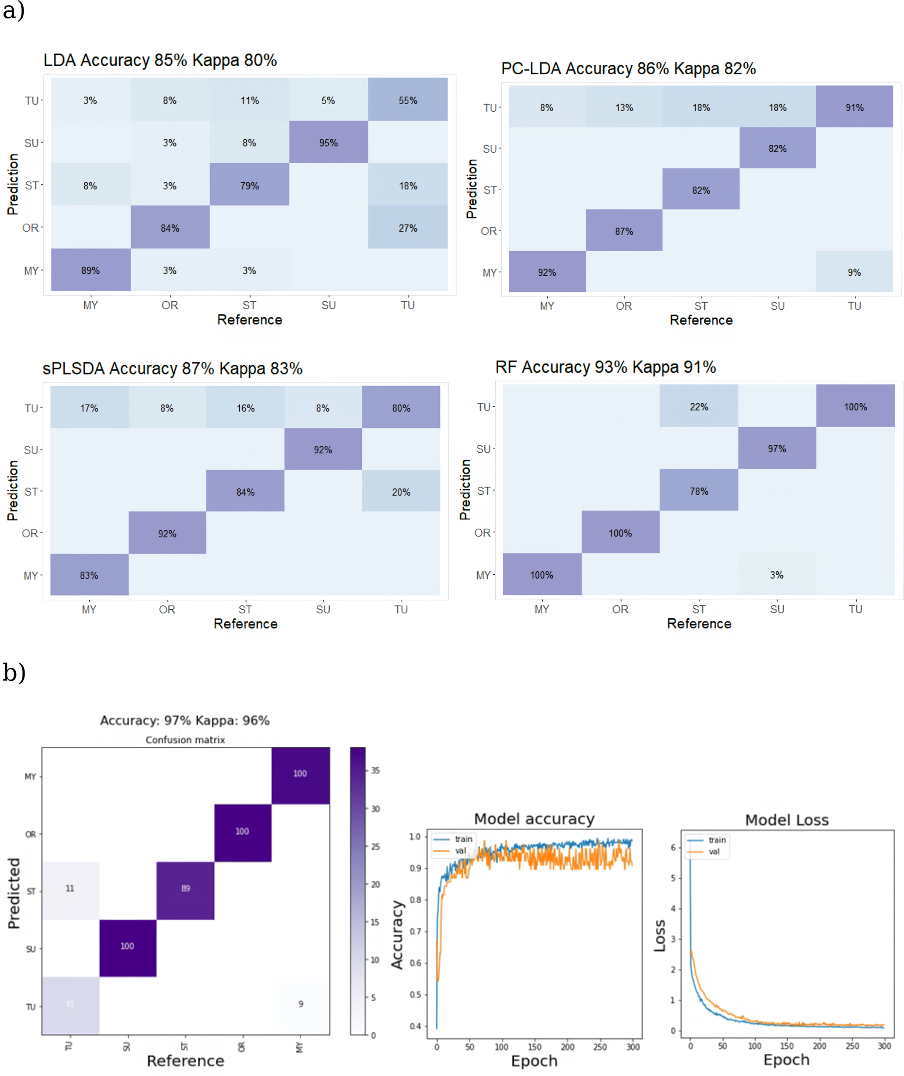
Figure 5a depicts the classification accuracy of the various trained models on the test data set as a confusion matrix that relates the predicted values to the ground truth. The confusion matrix is a cross table designed so that if the algorithm correctly predicts the real value of the test data, the value will fall on the diagonal, but incorrectly predicted or misclassified values will fall on either side of the diagonal. Normalized accuracy values are displayed as percentages in each category. The colors of the confusion matrix grids are proportional to the number of instances. Except for the TU class, the sample for each class of substitution group is balanced. Because kappa statistics (Cohen's kappa) corrects the bias of overall accuracy, including unbalanced class distribution, 75 it was employed as a cross-reference on classification results. Accuracy of class prediction of the test-set data by the LDA with no feature selection, as compared to the feature selection-based PC–LDA and sPLS–DA, the ensemble learning model RF and CNN are shown in Figure 5b.

Confusion table showing classification accuracy of trained models using Raman spectral data to categorize adulterated ground TU test samples. Panel (a) shows results from shallow ML algorithms (LDA, PC–LDA, sPLS–DA, and RF), while panel (b) displays outcomes from a DL 1D CNN. The right-side plot for 1D CNN depicts model accuracy and loss versus epoch during training and validation.
Feature selection strategies have increased the classification accuracy for Raman data (from 66% in LDA which performed poorly for this data set, versus 74% and 79% for PC–LDA and sPLS–DA, respectively) based on the overall accuracy values. The effect variable selection methods were less for FT-IR data sets where the accuracy achieved by LDA (85%) is slightly improved by PC–LDA (86%) and sPLS–DA (87%). For both Raman and IR spectral data sets, the overall classification accuracy achieved by RF was distinctly higher (93%). This result positions RF above the other shallow ML methods assessed in this study, aligning with the general view of RF as a high-performing ML algorithm. The prediction accuracy achieved by the 1D CNN implementation was 97% for both Raman and IR spectral data sets, surpassing all of the ML techniques tested for both data sets (Figures 5 and 6). The algorithm achieved 100% accuracy in predicting the classes of LC and all three azo dyes when using the Raman spectral data set, regardless of their level of substitution (Table II). The only misclassifications occurred between samples of TU and ST, both of which are plant-derived materials that closely resemble each other. The superior performance of the CNN model observed here is in line with the results reported in previous related research.48,76 The sample size to feature ratio of the data utilized in this study is small. To mitigate the issue of overfitting BN and dropout layers were implemented, which are recommended methods for addressing the issue of overfitting in DL models.34,76 By using these techniques, the model can better generalize to unseen data, despite the limited size of the data set. The application of a fivefold to 10-fold data augmentation, following the procedure described by Bjerrum et al., 34 did not result in any significant increase in the accuracy of predictions over the use of the un-augmented data set in this particular case (not shown). However, due to the time-consuming nature of processing the augmented data sets on a standard PC employed in this work, the impact of data augmentation on model performance was not thoroughly investigated. Comparison of model performance during training with and without Gaussian noise injection, BN, and dropout layers implementations indicated that the adoption of these regularization strategies positively affected model performance. The learning rate is an important tuneable hyperparameter in CNN. 77 While a low learning rate provides smooth convergence but may cause local minima rather than the global optimum, a high learning rate can accelerate learning but may impede convergence. 78 Finding the right hyperparameters is an iterative process that requires experience, but it can significantly reduce training time while enhancing performance. 79 Here, the model's accuracy showed improvement when an exponential step decaying learning rate 77 was utilized, and when a relatively larger batch size was used during model training. The greater variability evident in the validation curve of IR spectral data (Figure 6) indicates a potential concern with overfitting, especially when contrasted with the CNN model utilizing Raman data (Figure 5), despite previous efforts at regularization. This suggests that the IR data displayed more variability compared to its Raman counterpart. To improve the model's performance, future endeavors could explore additional measures, such as incorporating more training data and conducting a more meticulous fine-tuning of hyperparameters.
Confusion table showing classification accuracy of trained models using IR spectral data to categorize adulterated ground TU test samples. The remaining details are similar to the captions provided in Figure 5.
The classification metrics for the analysis of Raman and IR spectral data using both shallow ML algorithms (LDA, PC–LDA, sPLS–DA, and RF) and DL 1D CNN.

The table encompasses overall accuracy and precision, along with class-level performance. Accuracy signifies the overall correctness of predictions, precision indicates the proportion of true positives among predicted positives, Kappa reflects agreement beyond chance, and balanced accuracy ensures a balance between sensitivity (TP rate) and specificity (TN rate), especially crucial in imbalanced class scenarios.
The strong performance of the CNN model observed in this study, despite being trained on a relatively small data set, aligns with the idea that the sample size required for CNN model training is dependent on the model's complexity, the scope of the problem, and the characteristics of the data.27,29 The CNN results reported here were based on hyperparameter combinations that were deemed optimal during the training process. Although the CNN model achieved a higher accuracy than the parallel ML-based analyses, there is still scope for improving the model's performance, as there exist multiple methods for fine-tuning it. The use of a smaller research data set in conjunction with a simpler 1D CNN makes the method more accessible and ready to be tested for a wider range of research problems without requiring specialized computational resources. Simple 1D CNN experiments applied to spectrum data have shown superior results when compared to the shallow ML methods. Considering that the exploration of DL applications in food safety using IR spectroscopy is still in its early stages, the positive outcomes achieved thus far should be subject to further validation through additional research on this relatively novel approach.
Conclusion
This study assessed the effectiveness of both traditional chemometric algorithms and contemporary ML, and DL techniques based on 1D CNN in reducing dimensionality and improving the classification accuracy of ground TU samples adulterated with LC, azo-dyes (MY, OR, and SU III) and ST that are frequently cited as possible color enhancers and bulking agents. The unsupervised dimensionality reduction and pattern recognition performed using the nonlinear ML algorithm t-SNE in parallel with the standard linear-based PCA, revealed detailed patterns in the data that provided more insights into the data exploration process. A comparison of supervised classification analysis was performed between LDA, which considers the entire data set, feature selection-based PC–LDA and sPLS–DA; and RF, which is based on ensemble learning. The 1D CNN consistently demonstrates a higher classification accuracy trend, outperforming other algorithms in both Raman and FT-IR-based analyses, with RF closely following in multiple runs. This improved accuracy underscores the 1D CNN's proficiency in extracting meaningful features from complex spectral data. Furthermore, the 1D CNN distinguishes itself as the most efficient, undergoing training and testing on raw data, setting it apart from other compared algorithms. These capabilities suggest its potential to further empower spectroscopy in food safety research.
Footnotes
Acknowledgments
The author extends thanks to Todd Marrow, Director, and Jason Gotera, Supervisor, Canadian Food Inspection Agency, Greater Toronto Area Laboratory, for their encouragement and support. Gratitude to all manuscript reviewers. Special acknowledgment to Pavisha Kumaravel and Jeremy Van Buskirk for assistance in sample preparation and collecting IR spectra.
Declaration of Conflicting Interests
The author declared no potential conflicts of interest with respect to the research, authorship, and/or publication of this article.
Funding
The author disclosed receipt of the following financial support for the research, authorship, and/or publication of this article: This work was funded by the CFIA Technology Development (TD) Project (Project ID: P000427).