Sage Journals: Discover world-class research

Abstract

MicroRNAs (miRNAs) are a class of short noncoding RNAs that regulate gene expression through base pairing with messenger RNAs. Due to the interest in studying miRNA dysregulation in disease and limits of validated miRNA references, identification of novel miRNAs is a critical task. The performance of different models to predict novel miRNAs varies with the features chosen as predictors. However, no study has systematically compared published feature sets. We constructed a comprehensive feature set using the minimum free energy of the secondary structure of precursor miRNAs, a set of nucleotide-structure triplets, and additional extracted sequence and structure characteristics. We then compared the predictive value of our comprehensive feature set to those from three previously published studies, using logistic regression and random forest classifiers. We found that classifiers containing as few as seven highly predictive features are able to predict novel precursor miRNAs as well as classifiers that use larger feature sets. In a real data set, our method correctly identified the holdout miRNAs relevant to renal cancer.

Keywords

microRNA prediction feature selection classification

Introduction

MicroRNAs (miRNA) are small noncoding RNAs with an average length of 22 nucleotides (NTs).^1,2 MiRNAs are believed to play important roles in gene regulation by targeting the untranslated regions of messenger RNAs, which leads to cleavage or translational repression.^3–5 MiRNA sequences are encoded in the genome and are transcribed by RNA polymerases.⁶ The primary microRNA (pri-miRNA) transcript folds itself back to a typical hairpin secondary structure. The ribonuclease Drosha cleaves the pri-miRNA in the nucleus, resulting in the precursor miRNA (pre-miRNA). The length of the pre-miRNA differs from species to species, but has an approximate stem-loop length of 60–70 NTs.¹ Exportin-5 transports the pre-miRNA from the nucleus to the cytoplasm, where it is cleaved into about 22 NT duplexes (5’ and 3’). The mature miRNAs as well as the pre-miRNAs are conserved among several species.^1,6 The typical hairpin secondary structure is important due to the fact that it acts as a structural motif for Exportin-5,⁷ and also for Dicer to cleave the pre-miRNA into 5’ and 3’ mature miRNA.⁸

MiRNAs play an important role in human disease pathways⁹ and, due to the availability of high-throughput sequencing, it is advantageous to use computational methods to detect potential pre-miRNA sequences. In particular, studies have identified dysregulation of miRNAs as having a role in human cancers.¹⁰ Creating genome-wide miRNA expression profiles is an important step in uncovering such dysregulation cases in cancer subtypes. For example, renal clear-cell carcinoma accounts for approximately 90% of cases of kidney cancer in adults.¹¹ Due to the lack of reliable biomarkers indicating early stages of the disease, many patients develop metastases, leading to poor prognoses.¹² Survival rates significantly improve if these cancers are detected early.¹³ Recently, a study that used miRNA sequencing identified miRNAs differentially expressed in fresh-frozen, clear-cell renal cell carcinoma (ccRCC) versus nontumoral renal cortex cells.¹⁴ Computational miRNA prediction methods can reduce the high number of possible sequences that have to be biologically validated when analyzing miRNA profiles of cancer subtypes.

Previously published methods for predicting novel pre-miRNA sequences used different combinations of features and classifier algorithms, like Triplet Support Vector Machine (SVM),¹⁵ MiPred,¹⁶, and PmirP,¹⁷ among several other methods.

Xue et al.¹⁵ first proposed a method based on local contiguous structure composition centered on the middle nucleotide of each extracted structure triplet. These 32 nucleotide-structure triplets were used to train a SVM. MiPred implemented a random forest (RF) classifier using the same nucleotide-structure triplets as mentioned above.¹⁶ However, the authors added important feature characteristics of pre-miRNAs: the minimum free energy (MFE) of the secondary structure and the P-value of a randomization test to determine whether the energy is significantly different from those of randomly generated sequences. Zhao et al.¹⁷ used the left nucleotide, instead of the middle one, as the basis to create a set of 32 nucleotide-structure triplets and added features including information about the base pairings on the stem part of a pre-miRNA sequence. An overview of the feature sets in each study is shown in Table 1.

Table 1

Comparison of features in different selection methods.

METHOD	LEFT TRIPLET	MIDDLE TRIPLET	RIGHT TRIPLET	MFE SCORE	PERMUTATION ON MFE	NUMBER OF NTs IN STEM PARTS	NUMBER OF PAIRED NTS
Xue et al		√
Jiang et al		√		√	√
Zhao et al	√			√	√	√	√
Our method	√	√	√	√	√	√	√

Abbreviations: MFE, Minimum Free Energy; NT, Nucleotide.

In this study, we focus on the classification of real and pseudo pre-miRNAs using a new combination of features including a new variant of the nucleotide-structure triplets described in Xue et al.¹⁵ We use two machine-learning algorithms and validate the algorithms on completely unseen data, in contrast to most of the previous work. In addition, we test the performance of a minimal classifier, using only the most highly predictive features, and compare it to classifiers from previous studies.

Methods

Data set

All miRNAs that are biologically validated and published are stored in miRBase.^18–21 We downloaded the human pre-miRNA sequences from the release 18 in March 2012, which comprises 1,527 sequences. Only human pre-miRNAs, whose secondary structures contain one single loop, were considered, resulting in 1,478 sequences, which were used as a positive label set for classification. While a negative label set is required for a classifier training, no such data were available in public as negative results are seldom reported for novel miRNA discovery. We had to create a negative label set by ourselves. Using the process described in Xue et al.¹⁵ Jiang et al.¹⁶ and Zhao et al.¹⁷ protein-coding sequences (CDS) of human RefSeq genes without alternative splicing sites were downloaded from the UCSC Genome browser.²² We joined the CDS and extracted nonoverlapping segments, keeping the same length distribution of the current human real pre-miRNAs. To ensure that these pseudo pre-miRNA sequences had similar characteristics to the true miRNAs, the pseudo pre-miRNAs were filtered. The following criteria were used in the filter: the secondary structure contained only one single loop, the MFE of the secondary structure was at most -4.30, and the minimum number of base pairings at the stem was 14. We used these numbers because -4.30 is the maximum value of MFE in the true pre-miRNA set, and 14 is the minimum number of paired nucleotides in the stem part of the human real pre-miRNAs. In total, 21,836 pseudo sequences were generated and used as the negative sample set.

To train and validate the classifiers, we generated two data sets: a training and an external holdout set. The training set consisted of 1,183 true, positive-labeled pre-miRNAs and 17,469 negative samples from the set of pseudo pre-miRNAs. For validation, we used the remaining 295 positive and 4,367 negative instances. We also generated a validation set by holding out the top 30 differentially expressed miRNAs in the ccRCC miRNA expression data set (National Center for Biotechnology Information (NCBI) Gene Expression Omnibus (GEO) study ID: GSE37616¹⁴). These 30 were removed from the training data to test the ability to predict verified and biologically meaningful known miRNAs as if they were undiscovered.

Feature collection

We collected 115 different features related to the pre-miRNA sequence and its secondary structure. This is a superset of all features used in previous studies plus unused, novel features such as right-structure triplets. The features can be categorized into four classes: (1) MFE, (2) sequence, (3) secondary structure, and (4) a combination of sequence and secondary structure information. These classes and their feature values are described below in more detail.

Minimum free energy

The MFE is predicted by the Vienna RNAfold package.²³ Due to the fact that the energy value decreases with an increasing length of a pre-miRNA sequence, the MFE is also normalized by the length of the hairpin. To significantly distinguish random sequences from real ones based on the MFE value, a Monte Carlo randomization test (previously described in Bonnet et al.²⁴) was performed. For one given sequence, 1,000 random sequences were generated with the same dinucleotide distribution. The random doublet-preserving permutation algorithm²⁵ was used for the random sequence generation. The work described in Workman and Krogh²⁶ shows that random sequences with the same dinucleotide distribution are more likely to have similar MFEs than mononucleotide shuffled ones. A permutation score is calculated by R/(N + 1), where R is the number of randomized sequences that have a lower or equal MFE than the original one and N is the number of total random sequences.

Sequence information

The pre-miRNA contains sequence information about the 5’ and 3’ mature miRNAs. Given this information, knowing the full length of the pre-miRNA sequence becomes important. Based on the nucleotides in the pre-miRNA sequence, the GC ratio is also calculated as the proportion of bases G and C to all four bases (A, C, G, and T/U).

Nucleotide pairs

The secondary structures of the pre-miRNAs were predicted using the Vienna RNAfold package.^23,27 The structures are represented in bracket notation, which contains only two statuses for a nucleotide: paired and unpaired. Open and closed parentheses, “(”and”)”, are used for a nucleotide pair between a nucleotide on the 5’ end and a nucleotide on the 3’ end, respectively. Dots represent unpaired nucleotides. We did not distinguish between a nucleotide on the 5’ or 3’ end in this study, so we used “(” for both cases. A typical secondary structure of a pre-miRNA contains a stem and a single loop as displayed in Figure 1-a. Pre-miRNAs containing multiple loops in their secondary structures were not considered. The bracket notation gives information about the number of paired and unpaired nucleotides, as well as the ratio between them. The number of nucleotides on the 5’ and 3’ stem arm can be different due to bulges caused by unpaired nucleotides. This fact was used to normalize the number of nucleotide pairs by the longer stem arm. The loop part is normalized using the length of the pre-miRNA hairpin.

Figure 1.

The secondary structure of a pre-miRNA can change if one nucleotide is different. This Figure illustrates (A) the pre-miRNA hsa-miR-19b-1 sequence and its secondary structure, (b) a one-nucleotide change (yellow) that modifies the loop part, and (C) the stem arm.

It is important to encode the secondary structure with the sequence information because, as illustrated in Figure 1, the change of only one nucleotide in a pre-miRNA sequence can result in a different secondary structure. Due to this fact, the structure sequence in bracket notation is divided into overlapping triplets, considering each nucleotide in each triplet. For each base, there are 8 (2³) possible triplet structures: “…”, “.(”, “.(.”, “.((”, “(.”, “(.(”, “((.” and “(((”. With the left, middle, or right nucleotide of each triplet, there are 96 (4 (bases) x 8 (triplets) x 3 (different nucleotides)) possible nucleotide-structure combinations, which we list as “A…_l”, “A…_m”, “A…_r”, …, “U(((_l”, “U(((_m”, “U(((_r”, where “l,” “m,” and “r” represent left, middle, and right, respectively.

We only consider the 5’ and 3’ stem arm to extract the triplets from the secondary structure of a pre-miRNA, as shown in Figure 2. The numbers of different nucleotide-structure triplets are counted and then normalized by the number of the extracted triplets per nucleotide type (left, middle, or right) to generate a 96-dimensional feature vector.

Figure 2.

An overview of the workflow to extract different nucleotide-structure triplets.

Another characteristic of RNAs is the possible pairing of the bases G and U. These GU-wobble pairs are very common in RNAs, including miRNAs.²⁸ The normalized number of GU-wobble pairs (the total number normalized by the number of pairs) is also important because the number of GU-wobble pairs increases with the number of pairs in the hairpin.

Feature selection

We applied the RELIEF,²⁹ which is a feature selection method with tolerance and low (linear) computation cost, to rank features in terms of their contribution to the classification performance of the machine-learning model.

RELIEF uses a randomized mechanism to draw instances x and calculate their nearest hit (i.e., the closest same-class instances) and nearest miss (ie, the closest different-class instances) and adjust the weight vector on each feature using the following formula: $W_{i} = W_{i - 1} - {(x_{i} - h i t)}^{2} + {(x_{i} - m i s s)}^{2}$ where W is the weight of features and i the iteration cycle. That is, similar features of same-class instances will be assigned a lower weight, while similar features of different-class instances will be assigned a higher weight because they are discriminative.

Implementation

We used in-house Perl scripts to compile the real and pseudo miRNA sequences, extract the comprehensive set of features, and filter the sequences. We used the Weka³⁰ Java implementation of the RELIEF feature extraction algorithm. In-house R scripts were used for the creation of training and validation sets for each method, as well as the classifier training and evaluation. We used in-house-developed R functions and the R packages “randomForest”³¹ and “ROCR” for implementation.

Results

Selected features

Figure 3 shows RELIEF scores for selected features. We selected the top 30 features among the initial 115 using RELIEF scores. The number 30, chosen as the RELIEF curve, had a kink at 30 and this made our feature set size similar to those of comparing methods. We used 10-fold cross-validation to estimate the performance of the trained model. Consistent cross-validation performance shows a generalizability and lack of over-fitting with the model. We applied logistic regression (LR) and RF models to compare the performance of our feature set with other previously published feature sets. For a fair and comprehensive comparison, we used optimal parameters within each machine-learning method for each feature set (Table 2). Based on the slope change pattern in the RELIEF curve, we then selected the top 7 features to examine the performance of a “minimal” classifier as compared to more comprehensive feature sets.

Figure 3.

Feature contribution to outcome prediction according to the RELIEF score.

Table 2

Parameters used for RF for each feature set.

METHOD	NUMBER OF VARIABLES RANDOMLY SAMPLED AS CANDIDATES
Xue et al	6
Jiang et al	10
Zhao et al	10
Our method	5

Performance comparison of feature sets

The performance of the two classifier models with 10-fold cross-validation is illustrated in Table 3 and Figure 4. For classifier evaluation, we used the area under the ROC curve (AUC) as it is a well-known aggregated discrimination performance measure that does not commit to a particular threshold.³² Our feature set combination shows consistently higher AUC values than the feature sets of Xue et al.¹⁵ and comparable AUC values to those published by Jiang et al.¹⁶ and Zhao et al.¹⁷ in both types of classifiers (LR and RF). We also used a holdout set of 20% of the data for external validation. The AUC values resulting from the use of the classifiers on this unseen data were slightly higher (Table 4) than they were in the training set, indicating low likelihood of over-fitting. Figure 4 shows the estimated AUC values for each feature set applied to the LR and RF models. Given the similarity in discrimination among the last three methods–Jiang, Zhao, and the proposed method–we investigated to identify the common features across all three methods that are most critical for prediction. Based on the RELIEF score, we selected the top seven common features and trained LR and RF. The “minimal” classifiers reached the same performance level as the ones with features more than seven, with AUC values of 0.9824 and 0.9796 for LR and RF, respectively, on the validation set. In addition, we confirmed the robustness of the RELIEF selections by sequentially adding features onto a RF classifier based on the RELIEF scores (Fig. 6).

Table 3

Average performance of different feature sets and classifier models in 10-fold cross-validation.

METHOD	AUC LR	95% CI FOR LR	AUC RF	95% CI FOR RC
Xue et al	0.9499	(0.9442, 0.9556)	0.9217	(0.9128, 0.9306)
Jiang et al	0.9706	(0.9658, 0.9755)	0.9688	(0.9627, 0.9748)
Zhao et al	0.9752	(0.9688,0.9817)	0.9679	(0.9606, 0.9753)
Our method	0.9759	(0.9730, 0.9789)	0.9716	(0.9659, 0.9772)

Figure 4.

Performance of two classifier models on the validation set: (A) LR and (B) RF.

Table 4

Performance of different feature sets and classifier models on the external validation data set.

METHOD	AUC LR	AUC RF
Xue et al	0.9651	0.9304
Jiang et al	0.9805	0. 9748
Zhao et al	0.9844	0. 9745
Our method	0.9861	0.9786

Figure 6.

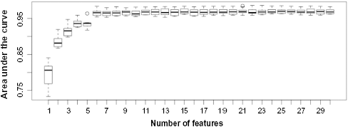
AUC values versus number of features sequentially added based on RELIEF score for RF classifiers in a 10-fold cross-validation.

Real data miRNAs

Our feature set and that of Jiang et al.¹⁶ had equal sensitivity (0.9) at a threshold of 0.5, while those of Xue et al.¹⁵ and Zhao et al.¹⁷ had sensitivities of 0.067 and 0.633, respectively, on the holdout true-positive miRNA set from the renal cancer study. In a histogram of prediction probabilities (Fig. 5), our feature set exhibited a skewed distribution at high-valued output estimates, indicating that, when the classifiers that use our feature set output a high score, there is high likelihood that this is a true miRNA. Of interest are a few real miRNAs that had low scores (below 0.5) for all feature sets. None of the feature sets were able to predict hsa-miR-660, hsa-miR-15a, and hsa-miR–532. miRBase¹⁹ stem-loop diagrams show that all three of these miRNAs have noncanonical two-loop structures, which cause all the feature sets to fail.

Figure 5.

Histogram of estimates (ie, prediction probabilities) for the positive samples from the renal cancer study.

Discussion

We compared our minimal feature set with information about the sequence and structure of a pre-miRNA with three other published feature sets. An important characteristic that defines real pre-miRNA sequences is the MFE. Adding this energy value to a feature set increased the prediction performance, regardless of the classifier model. This was verified through the similar performance of all methods that use MFE, including ours, Jiang,¹⁶ and Zhao.¹⁷

Previously, other methods have relied on nucleotide triplets to contain the sequence and structure information used to accurately predict pre-miRNAs. A single-nucleotide change can have a significant impact on the secondary structure, so these features were useful for capturing these characteristics of miRNAs. MFE values were added to improve classifier performance, based on studies on the MFE of noncoding RNAs which determined that pre-miRNAs have lower free energy than randomized sequences, while other ncRNAs do not.²⁴ After comprehensive evaluation, we find that with MFE and base pairing counts, the fine-grain information from nucleotide triplet features is no longer needed. Since the sequence is used to determine the secondary structure in the first place through the Vienna RNAfold package, the resulting MFE and aggregate base pairing information already contain this critical information used to classify pre-miRNAs. This discovery allows us to create the minimal classifier for pre-miRNA prediction using biologically explainable, structure-wide features. The increased ease in implementation of this classifier makes it a good baseline for the creation of more sophisticated methods to predict noncanonical miRNAs and other ncRNAs.

A limitation of this work is in the scope of questions addressed. We analyzed a comprehensive set of miRNA features to identify the importance of top features and compared the results among similar feature sets. We also tested the ability of the sets to identify biologically relevant renal cancer miRNAs as if they were undiscovered in order to assess the ability of the feature sets to predict truly novel miRNAs. However, our method may still have limited ability to accurately predict noncanonical miRNAs.

The two paths for extension of this work are applying more advanced machine-learning methods on our feature set and applying our feature set to identify novel miRNAs in additional data sets. Issues such as creating the artificial negative data sets, class imbalance between the negative and the positive training data, and addition of features and methods to identify noncanonical miRNAs were outside of the scope of this work, yet may be useful in improving the accuracy of miRNA prediction methods.

Conclusion

We compared feature sets in classifier performance for the task of predicting novel pre-miRNAs. A minimal set of seven is sufficient to attain the same classification performance as more comprehensive feature sets. Further validation using other data sets will help determine whether the number and type of features is generalizable to precursor miRNAs found in different types of samples.

Author Contributions

PS and JK conceived and designed the experiments. PS, EL, and JK analyzed the data. PS and EL wrote the first draft of the manuscript. PS, EL, JK, XJ, and LOM contributed to the writing of the manuscript. PS, EL, and JK jointly developed the structure and arguments for the paper. PS, EL, JK, XJ, and LOM agreed with manuscript results and conclusions. JK and LOM made critical revisions. All authors reviewed and approved of the final manuscript. We thank Tyler Bath for proofreading the manuscript.

References

Bartel

D.P.

. MicroRNAs: genomics, biogenesis, mechanism, and function. Cell. 2004; 116(2): 281–97.

Ambros

, Bartel

D.P.

. A uniform system for microRNA annotation. RNA. 2003; 9(3): 277–9.

Kim

V.N.

, Nam

J.W.

. Genomics of microRNA. Trends Genet. 2006; 22(3): 165–73.

Winter

, Jung

, Keller

, Gregory

R.I.

, Diederichs

. Many roads to maturity: microRNA biogenesis pathways and their regulation. Nat Cell Biol. 2009; 11(3): 228–34.

Hinske

L.C.

, Galante

P.A.

, Kuo

W.P.

, Ohno-Machado

. A potential role for intragenic miRNAs on their hosts’ interactome. BMC Genomics. 2010; 11: 533.

Westholm

J.O.

, Lai

E.C.

. Mirtrons: microRNA biogenesis via splicing. Biochimie. 2011; 93(11): 1897–904.

Zeng

, Cullen

B.R.

. Structural requirements for pre-microRNA binding and nuclear export by Exportin 5. Nucleic Acids Res. 2004; 32(16): 4776–85.

Zhang

, Kolb

F.A.

, Jaskiewicz

, Westhof

, Filipowicz

. Single processing center models for human Dicer and bacterial RNase III. Cell. 2004; 118(1): 57–68.

Lussier

Y.A.

, Stadler

W.M.

, Chen

J.L.

. Advantages of genomic complexity: bioinformatics opportunities in microRNA cancer signatures. J Am Med Inform Assoc. 2012; 19(2): 156–60.

10.

Croce

C.M.

. Causes and consequences of microRNA dysregulation in cancer. Nat Rev Genet. 2009; 10(10): 704–14.

11.

Devesa

S.S.

, Silverman

D.T.

, McLaughlin

J.K.

, Brown

C.C.

, Connelly

R.R.

, Fraumeni

J.F.

Jr . Comparison of the descriptive epidemiology of urinary tract cancers. Cancer Causes Control. 1990; 1(2): 133–41.

12.

Ramana

. RCDB: renal cancer gene database. BMC Res Notes. 2012; 5: 246.

13.

Pantuck

A.J.

, Zisman

, Belldegrun

A.S.

. The changing natural history of renal cell carcinoma. J Urol. 2001; 166(5): 1611–23.

14.

Osanto

, Qin

, Buermans

H.P.

. Genome-wide microRNA expression analysis of clear cell renal cell carcinoma by next generation deep sequencing. PLoS One. 2012; 7(6): e38298.

15.

Xue

, Li

, He

, Liu

G.P.

, Li

, Zhang

. Classification of real and pseudo microRNA precursors using local structure-sequence features and support vector machine. BMC Bioinformatics. 2005; 6: 310.

16.

Jiang

, Wu

, Wang

, Ma

, Sun

, Lu

. MiPred: classification of real and pseudo microRNA precursors using random forest prediction model with combined features. Nucleic Acids Res. 2007; 35(Web Server issue): W339–44.

17.

Zhu

, Zhao

, Xu

. mirTools: microRNA profiling and discovery based on high-throughput sequencing. Nucleic Acids Res. 2010; 38(Web Server issue): W392–7.

18.

Griffiths-Jones

. The microRNA registry. Nucleic Acids Res. 2004; 32(Database issue): D109–11.

19.

Griffiths-Jones

, Grocock

R.J.

, van Dongen

, Bateman

, Enright

A.J.

. miRBase: microRNA sequences, targets and gene nomenclature. Nucleic Acids Res. 2006; 34(Database issue): D140–4.

20.

Kozomara

, Griffiths-Jones

. miRBase: integrating microRNA annotation and deep-sequencing data. Nucleic Acids Res. 2011; 39(Database issue): D152–7.

21.

Griffiths-Jones

, Saini

H.K.

, van Dongen

, Enright

A.J.

. miRBase: tools for microRNA genomics. Nucleic Acids Res. 2008; 36(Database issue): D154–8.

22.

Karolchik

, Baertsch

, Diekhans

. The UCSC genome browser database. Nucleic Acids Res. 2003; 31(1): 51–4.

23.

Lorenz

, Bernhart

S.H.

, Höner Zu Siederdissen

. Vienna RNA Package 2.0. Algorithms Mol Biol. 2011; 6: 26.

24.

Bonnet

, Wuyts

, Rouze

, Van de Peer

. Evidence that microRNA precursors, unlike other non-coding RNAs, have lower folding free energies than random sequences. Bioinformatics. 2004; 20(17): 2911–17.

25.

Altschul

S.F.

, Erickson

B.W.

. Significance of nucleotide sequence alignments: a method for random sequence permutation that preserves dinucleotide and codon usage. Mol Biol Evol. 1985; 2(6): 526–38.

26.

Workman

, Krogh

. No evidence that mRNAs have lower folding free energies than random sequences with the same dinucleotide distribution. Nucleic Acids Res. 1999; 27(24): 4816–22.

27.

Hofacker

I.L.

, Fontana

, Stadler

P.F.

, Bonhoeffer

L.S.

, Tacker

, Schuster

. Fast folding and comparison of RNA secondary structures. Monatsh Chem. 1994; 125(2): 167–88.

28.

, Lv

, Wong

C.K.

. The effect of central loops in miRNA: MRE duplexes on the efficiency of miRNA-mediated gene regulation. PLoS One. 2008; 3(3): e1719.

29.

Kira

, Rendell

L.A.

. The feature selection problem: Traditional methods and a new algorithm. Proceedings AAAI-92, San Jose, CA, MIT Press, Cambridge, MA (1992), pp. 129–34.

30.

Hall

, Frank

, Holmes

, Pfahringer

, Reutemann

, Witten

I.H.

. The WEKA data mining software: an update. ACM SIGKDD Explor Newsl. 2009; 11(1): 10–8.

31.

Liaw

, Wiener

. Classification and regression by randomForest. R News. 2002; 2(3): 18–22.

32.

Flach

, Hernández-Orallo

, Ferri

. A coherent interpretation of the AUC as a measure of aggregated classification performance. In: Proceedings of 28th International Conference on Machine Learning, Bellevue, WA, USA. 2011; pp. 657–64.