Sage Journals: Discover world-class research

Abstract

Driver assistant systems enhance traffic safety and efficiency. The accurate 3D pose of a front vehicle can help a driver to make the right decision on the road. We propose a novel real-time system to estimate the 3D pose of the front vehicle. This system consists of two parallel threads: vehicle rear tracking and mapping. The vehicle rear is first identified in the video captured by an onboard camera, after license plate localization and foreground extraction. The 3D pose estimation technique is then employed with respect to the extracted vehicle rear. Most current 3D pose estimation techniques need prior models or a stereo initialization with user cooperation. It is extremely difficult to obtain prior models due to the varying appearance of vehicles' rears. Moreover, it is unsafe to ask for drivers' cooperation when a vehicle is running. In our system, two initial keyframes for stereo algorithms are automatically extracted by vehicle rear detection and tracking. Map points are defined as a collection of point features extracted from the vehicle's rear with their 3D information. These map points are inferences that relate the 2D features detected in following vehicles' rears with the 3D world. The relative 3D pose of the onboard camera to the front vehicle rear is then estimated through matching the map points with point features detected on the front vehicle rear. We demonstrate the capabilities of our system by testing on real-time and synthesized videos. In order to make the experimental analysis visible, we demonstrated an estimated 3D pose through augmented reality, which needs accurate and real-time 3D pose estimation.

Keywords

3D pose estimation vehicle rear tracking driver assistance system

1. Introduction

Vehicle crashes occur every minute around the world. This makes vehicle collisions the leading cause of severe injuries worldwide, according to the report of the World Health Organization. With the aim of reducing the number of injuries and accident severity, crash-prevent systems is becoming an area of active research among automotive manufacturers, suppliers and universities. An onboard driver assistance system aiming to provide the driver with a 3D pose of front vehicles is very attractive. Besides preventing collisions, the accurate pose of the front vehicle can help a driver to make the right decisions on the road. This task includes two steps: front vehicle detection and 3D pose calculation.

Figure 1.

Current vehicle detection methods

Vision-based vehicle detection has received considerable attention over the last 20 years. As shown in Fig.1, these applications are grouped into two general categories, depending on the installation location of the camera: one is a fixed camera which is installed roadside; the other one is a camera mounted on a vehicle. For vehicle detection with a roadside camera, many vehicle detectors utilize background subtraction methods [1, 2]. Wu et al. [1] proposed a grey-level differential value method to dynamically segment moving objects from the background. This method rests on the assumptions that road surfaces are grey, lane marks are yellow or white and that the remaining colours are to be regarded as moving objects on the road. Vargas et al. [2] integrated a background subtraction algorithm with a sigma-delta filter, which has high computational efficiency. The proposed method attempts to achieve a background updating model at the pixel level by introducing a confidence measurement for each pixel.

Figure 2.

Comparison between background subtraction techniques with a road-side camera and an onboard camera

For vehicle detection with an onboard camera, however, background subtraction cannot be easily used because prior knowledge about the background is not available. For example, we achieve good results - as shown in Fig. 2(a) - with a road-side camera using the background subtraction algorithm in [2]. However, this result cannot be obtained when we use the same algorithm with an onboard camera - as shown in Fig. 2(b) - because the background is not static. The processing speed is extremely critical in onboard vehicle detection systems, since the prompt feedback from such a system could save time for a driver's reaction. Various approaches with low computational costs have been proposed in the literature, which can be classified into one of the following categories: appearance-based analysis [3 –12] and low-level-based features [13 –16]. Tai et al. [10] used an active contour method with a Kalman filter to detect and track vehicles. As demonstrated in their research, the vehicles could be easily tracked with a low computation loading. However, the contour initialization posed a critical risk. Chu et al. [8], Du et al. [3]and Hofmann et al. [9] reported that vehicles rear or frontal views are generally symmetrical in both horizontal and vertical directions. However, an important issue arises when computing symmetry from image intensity in that symmetry is quite prone to false detection, such as symmetrical background objects or partly occluded vehicles. It was observed that the rear or frontal views of vehicles usually contain many horizontal and vertical structures, such as rear windows and bumper; thus, Betke et al. [5] proposed a coarse-to-fine method to detect distant cars via searching for rectangular objects. A refined search was activated only for small regions on the image, after a whole image search. Within a predefined maximum distance from the detected road lanes, Bucher et al. [7] found vehicle candidates with edge features by scanning the image from the bottom up to a certain vertical position, line-by-line. Although fast and positive results were made, the method very attractive, its performance and robustness strictly depended on well-tuned parameters, such as the thresholds for detecting edges and choosing the most important vertical and horizontal edges. In addition, the use of vehicle lights as another clue for vehicle detection was studied. Malley et al. [12]detected and tracked vehicles by segmenting rear-facing lamps based on a red-colour threshold. Meanwhile, Cucchiara et al. [6] employed a morphological analysis to detect vehicle light pairs in a narrow inspection area. This kind of method was very sensitive to illumination, whereas promising results could only be obtained at night. Shadow information as a sign pattern for vehicle detection was investigated in [4, 11]. Liu et al. [11] distinguished vehicle candidates using the shadow underneath a vehicle. Tzomaks et al. [4] analysed the grey level around the detected lanes to segment shadow and then found a vehicle. However, there is no systematic way to choose the appropriate threshold values for shadow segmentation.

Texture patterns have also been used for vehicle detection. These texture patterns were usually presented by low-level features, such as feature points [15, 16], eigenvalues [13] and Haar-like features [14], etc., rather than the structure features described above. Arai et al. [15] proposed a vehicle detection system based on the shift of a feature plane, which was constituted by feature points on the front surface of the vehicle. They found the feature plane of the vehicle's front surface shifts in accordance with an affine transform. Jazayeriet et al. [16] extracted low-level features, such as corners, intensity peaks and horizontal line segments from images. These features were profiled to the temporal space. To identify tracked features, such as a car or a background, they estimated probability distributions for the motion properties of cars and the background. The Hidden Markov Model (HMM) was used to separate vehicles from the background and track them probabilistically. At the same time, a statistical model was used in [13], performing vehicle detection by Principal Component Analysis (PCA). Negri et al. [14] compared the performances of different vehicle detectors. In their study, these detectors were trained from Haar-like features, a histogram of oriented gradient features and a fusion of the two features sets, respectively. Subsequently, the best performance was achieved by the feature fusion. The low-level feature-based methods usually consist of feature extraction and classifier training. It is worth mentioning that in view of the various appearances of vehicles it is normally extremely difficult to construct explicit models.

Another interesting method was raised by Arrospide et al. in [17]. They found a vehicle via ground plane detection. The proposed method is based on the reliable estimation of the homography between ground planes in successive images. The homography calculation is grounded on a linear estimation framework, which predicates the ground plane transformation matrix while it is dynamically updated with new measurements. Disappointingly, the results showed the speed of the method to be only around 10fps, with an image resolution of 360*288, as implemented on a 2GHz 2GB Memory PC.

To the best of knowledge - with notable exceptions like [18 –21] - most of the previous vehicle detection works have been 2D. Even in [22], a proposed pre-crash system was based on vehicle rear detection in a 2D rather than a 3D space. With an onboard camera, Zielke et al. [18] measured the distance from front vehicles under a Time-to-Collision (TTC) model. This TTC model was represented by the distance between two images points on the rear surface of the front vehicle and the rate of the changing rate for this distance. However, this proposed method strictly rested on the assumption that the vehicle with the camera is moving up to the front vehicle rear vertically, which cannot be guaranteed in reality. Besides this, the stable detection and tracking of the two points in the marker-less scene was very difficult. Broggi et al. [20] and Bensrhair et al. [19] detected and localized a front vehicle using stereo vision. With known stereo rig parameters, a 3D map of the viewed scene can be constructed via the differences in the corresponding pixels between left and right images. Though this method can obtain accurate measurements, it is extremely time-consuming. Kim et al. [21] used a sonar sensor for vehicle detection and distance estimation. Although these non-visual sensors can measure distance directly, without requiring powerful computing resources, they have several drawbacks, such as a high cost, a low spatial resolution and a slow scanning speed. Furthermore, visual information is very important in a number of related applications, such as lane detection and traffic sign recognition.

In this paper, our proposed approach recognizes and tracks vehicle rears quickly based on license plate localization. Then, a 3D pose is estimated with respect to the extracted vehicle rear. This has several advantages: 1, a license plate (LP) is smaller and much more standardized than a vehicle rear, making LP localization quicker and more robust than directly detecting a vehicle; 2, because only the region around the LP rather than the whole vehicle is required for 3D pose estimation, we are able to achieve real-time performance; 3, pose measurement is not affected, even when the extracted regions of a vehicle's rear in successive frames are not exactly the same, since vehicle's rear are considered as planar.

The remainder of this paper is structured as follows: we begin by reviewing the related work about 3D pose estimation from a planar object in section 2. In section 3 we present an overview of our own system. Subsequently, section 4 interprets the process of map initialization. Next, vehicle rear detection, tracking and pose estimation are described in section 5. In section 6 we present map updates and maintenance in detail. The experimental results are demonstrated in section 7. Finally, we conclude in section 8.

2. Related Work about 3D Pose Estimation from a Planar Target

There are several approaches for pose estimation, where the 6 degrees of freedom of a camera's pose are calculated from correspondences between images and the real scene structure. Most of them work with the theory that the pose of a calibrated camera can be uniquely estimated by no less than four coplanar and no collinear points. Depending on how correspondences between images and the real world should be established, these methods could be divided into two categories: prior knowledge-based methods and self-initialization-based methods.

With the prior model, the registration between an image and the real world can be performed directly. The camera pose can then be estimated from these corresponding points [23 –25]. Drummond et al. [24] found camera poses that correctly re-project some fixed features of a prior 3D model into the 2D image. These features can be edges, line segments or points. Through the least-squares minimization of an error function, the best pose was found. Actually, a comprehensive prior model is not readily available. Some researchers have established a relationship between images and the real world using fiducial markers. For instances, Kawano et al. [23] discussed a number of planar markers for Augmented Reality (AR). The salient markers with known pose information in the real world were easily detected in the images. Meanwhile, Mondragon et al. [25] utilized 3D pose estimation techniques in Unmanned Aerial Vehicle (UAV) control. Specifically, their proposed method asked a UAV driver to select four points on the image that correspond to four corners on the helipad.

Normally, 3D pose estimation implements a previously unknown scene without any known models. This problem was solved in [26, 27] by building an initial map from a five-point stereo [28]. Mouragon et al. [26] tracked a camera using local bundle adjustment over the most recent camera poses and obtained accuracy over a long distance. Klein et al. [27] established a small AR workspace where the user will spend most of their time. As such, they built a long-time map in which features were constantly re-visited. This is similar to our own case, in which we focus on the extracted vehicle rear region. User cooperation is required in [27] for map initialization; however, it would be unsafe to ask a driver to manipulate this. In our method, the initial map is constructed with feature points tracked on two extracted vehicle rear regions at the beginning.

3. Method Overview

As shown in Fig. 3, our system consists of two threads: tracking and mapping. Although these two threads are intimately linked, most of the time they perform in parallel in order to save processing time. For a mapping thread, as shown in Fig. 3, and given the assumption that vehicle rears are detected and tracked on frames, a map is initialized from feature point correspondences found in the first two keyframes. The map consists of a collection of point features with their 3D information. Each map point has a coordinate in the world coordinate system, references to the source keyframe and to the patch source pixels. The map is updated by keyframes, rather than frame by frame. These map points can be considered as a “bridge”, which relate image points to the real world.

For a tracking thread, and with the assumption that the map has been already initialized, video is captured by the camera mounted on the front of the vehicle. Because we only need information of the front vehicle rather than the whole image, we only process a Region of Interest (ROI), as shown in Fig.4. The size of the ROI in our experiment is 640*480 pixels. A rejection cascade of an Adaboost classifier with line segment features and Haar-like features [29] is utilized in order to find a set of LP candidates quickly. A best detection is obtained, followed by non-maximal suppression. Based on a localized LP, a vehicle rear is extracted. FAST (Features from Accelerated Segment Test) corners [30] are then detected on the extracted vehicle rear. After finding correspondences between the detected features and map points, the relative pose of the camera to the map is calculated.

Figure 3.

Method overview

Figure 4.

ROI on the whole frame

4. Map Initialization

As indicated in [26], the motion between two consecutive frames must be large enough to compute the epipolar geometry. For map initialization, we select two frames at the beginning, relatively far from each other but with enough matched points. The first extracted vehicle rear is selected as a keyframe K. In the next N detected vehicle rears, we choose the second keyframe that is furthest from K and with the most matched interest points with K. In our experiments, we choose the shortest distance, which is 20 pixels, and the least number of matched points, which is 100.

As shown in Fig.5, after obtaining the first two keyframes, map initialization is done with a five-point algorithm [17] and RANSAC [31]. First, the essential matrix E between the two keyframes is calculated from a sample of 5 point correspondences:

\begin{array}{l} q_{1}^{i} ​^{T} E q_{2}^{i} = 0, i \in {1 \dots 5} \\ E E^{T} E - \frac{1}{2} t r a c e (E E^{T}) E = 0 \end{array}

(1)

Where $q_{1}^{i}$ and $q_{2}^{i}$ are the 5 points projections on the two keyframes, respectively. At most, 10 solutions for E could be obtained from (1). Each E produces a solution for the camera's pose. We first discard the poses for which at least one of the 5 points is not reconstructed in front of the camera. Next, the remaining solutions for the camera pose are filtered with a RANSAC approach: a sample set of five points are selected to hypothesize a number of cameras' poses while the remaining matched points are tested for consensus. The best camera pose is chosen by computing the re-projection error over all the possible camera poses for all of the remaining matched points and keeping that with the highest number of matches. A map coordinate is constructed in such a way that the X axis and the Y axis are on the vehicle rear plane, while the Z axis is perpendicular to the vehicle rear plane.

Figure 5.

Map initialization

Figure 6.

Constructed map and keyframes

As shown in Fig.6, each map point refers to a single source keyframe, where the map point first takes place. For example, the map points generated in the procedure of map initialization refer to the first keyframe. The relative 3D pose between the map point and its source keyframe are also recorded. Furthermore, each map point refers to its absolute 2D location on the source keyframe. FAST corners, as image features, are detected in our method as 8*8 pixel squares on greyscale frames. The centres of these pixel patches are recorded as the absolute 2D locations. Finally, because the sizes of the extracted vehicle rears change frame by frame, the relative 2D location of the map point on the source keyframe is also recorded, $(\frac{x}{W v}, \frac{y}{H v})$ , where $(x, y)$ is an absolute 2D location of the map point on the source vehicle rear frame and $(w_{v}, H_{v})$ is width and height of the extracted vehicle rear.

5. Vehicle Rear Detection, Tracking and 3D Pose Estimation

This section describes the procedure for vehicle rear detection, tracking and 3D pose estimation. In order to allow the reader to follow the idea of our method more easily, we present a procedure for map initialization initially in the last section - which actually works in parallel with steps in this section. Therefore, the contents in this section build on the assumption that a map of 3D points has already been constructed.

5.1. Vehicle rear detection

For vehicle rear extraction, we need to localize LPs quickly and accurately. For LP detection, many researchers [32, 33] used AdaBoost in conjunction with Haar-like features. Compared with other pixel-level features, Haar-like features save considerable computational costs since they are extracted from integral representations of an image rather than from individual pixels. However, Haar-like features are very sensitive to illumination and the selected feature set has a very large dimension, which makes the training process very time consuming and the classifying process unstable. In our system, we introduce line segment features, namely the density ( $L_{D}$ ), directionality ( $L_{d i}$ ) and regularity ( $L_{R}$ ) of line segments extracted from an image. After applying edges-detection on an LP-included image, we can obtain dense vertical strokes inside an LP region as line segments. The properties of line segment features are described as follows:

{\begin{matrix} L_{D} = n_{(l i n e)} / N_{(b l o c k)} \\ L_{d i} = N_{(θ_{v})} / N_{(θ_{l})} (80^{\circ} \leq θ_{v} \leq 100^{\circ}, 0^{\circ} \leq θ_{l} \leq 179^{\circ}) \\ L_{R} = s t d {γ} / m e a n {γ} \end{matrix}

(2)

As shown in Fig.7, $n_{(l i n e)}$ is the number of line segments in a block while $N_{(b l o c k)}$ indicates the size of a block by the number of pixels in it. It tends to have a high density of line segments in the LP region. Moreover, rather than being disorderly, line segments inside an LP are prone to be approximately vertical. We utilize directionality ( $L_{d i}$ ) to describe this pattern of line segments. We refer to Fig. 7(e), where θ is the angle between the vertical axis (y-axis) and the perpendicular of line segment. The line segment with θ within the range [80, 100] is regarded as a vertical stroke. As shown in Fig. 7(e), both $l^{1}$ with $θ^{1}$ and $l^{2}$ with $θ^{1}$ are considered as vertical strokes. $N_{(θ_{v})}$ is the number of vertical line segments in a block while $N_{(θ_{l})}$ is the number of all line segments in it. The LP region should have a high value for $L_{d i}$ . Finally, regularity is introduced to measure the regular repetition of line segments inside LP. ${γ}$ is the inter-distances of the vertical line segments in a block. The smaller the value of R indicates the greater the regularity of the block. The localized LP is shown as a red rectangle in Fig. 7.

Figure 7.

Line segment feature for license plate localization

After integrating line segment features into a traditional cascade of an Adaboost classifier with Haar-like features, we can dramatically drive down the amount of required Haar-like features - from 412 in the traditional method to 180 in our experiment - as well as the training time. With a rejection cascade consisting of 13 nodes, as illustrated in Fig. 8, a set of LP candidates are detected. We choose the fittest one after implementing non-maximal suppression. Since we consider the vehicle rear as a plane, only a part of the vehicle rear is required for 3D pose estimation. We extract a vehicle rear as Wv=4*W and Hv=3*H, where Wv and Hv are the width and the height of the vehicle rear and W and H are the width and the height of the localized LP, respectively.

Figure 8.

Rejection cascade trained from line segment features and Haar-like features

5.2. Update search region for the license plate

The region prediction of the LP in the next frame is important. We use an alpha-beta filter to predict the possible region for the LP. It resembles a Kalman filter but is less complex and has less parameters to tune, having only alpha and beta values. The alpha controls the response to a new pose input while the beta controls how responsive the filter is to a new velocity input. The alpha and beta gains range from [0, 1]. The alpha-beta filter update is as follows:

\begin{array}{l} r_{t} = X_{t} - {\overset{\land}{X}}_{t - 1} \\ {\overset{\land}{X}}_{t} = {\overset{\land}{X}}_{t - 1} + α r_{t} \end{array}

(3)

where ${\overset{\land}{X}}_{t}$ is the current smoothed out pose estimation, ${\overset{\land}{X}}_{t - 1}$ is the previous estimation, $X_{t}$ is the pose input, $r_{t}$ is the residual and α is the gain.

5.3. Establishment of the correspondence between map points and frame points

For camera pose estimation, we need to find interest points on the current frame and match them up with map points. As described in the section on map initialization, after transferring the extracted vehicle rear to grey scale, we run the FAST corner detector on it. Each FAST feature vector describes an 8*8 image patch. To match the map points with the detected points on the current frame, we use a K-Means tree. The match is performed in a binary tree by comparing which centroid is closer to the query and going down the tree. The final leaf node will contain a handful of features that have to be searched linearly. Some matches will not be one to one correspondences when more than one FAST feature points to the same map point. To resolve this conflict, the FAST feature with the highest matching score is kept. To promote match accuracy, we perform a fix-range image search on the current frame. For every map point, we search on the current vehicle rear as:

\begin{array}{l} s e a r c h c e n t e r = (\frac{x}{W v} w_{v}', \frac{y}{H v} H_{v}') \\ s e a r c h p a t c h = \frac{1}{8} w_{v}' \times \frac{1}{16} H_{v}' \end{array}

(4)

where $(\frac{x}{W v}, \frac{y}{H v})$ is described in the section of map initialization as the relative location of the map point on the source keyframe and $w_{v}'$ and $H_{v}'$ are the width and height of the current vehicle rear, respectively.

5.4. The camera project model and pose estimation

To estimate camera pose, we should understand that the camera model points in the world coordinate are projected onto an image frame after being projected onto a camera-centred coordinate. The following equation describes the projection onto the camera-centred coordinate:

\begin{array}{l} p_{i C} = E_{C W} P_{i W} \\ E_{C W} = - R^{T} T, \\ T = [t_{x}, t_{y}, t_{z}], R=[θ, ψ, φ] \end{array}

(5)

where $P_{i W}$ is a point in a world coordinate, $p_{i C}$ is a transformed point in a camera-centred coordinate, $E_{C W}$ is a 3*3 transform matrix that contains a translation T and a rotation R.

To transfer the point $p_{i C}$ on a camera-centred coordinate to a point $p_{i}$ image, the camera's intrinsic parameters are required. We obtain these parameters by camera calibration. A calibrated camera projection model is as follows:

\begin{array}{l} C a m P a r a s = [f_{x}, f_{y}, x, 0 y_{0}, ω] \\ (\begin{matrix} x \\ y \end{matrix}) = (\begin{matrix} x_{0} \\ y_{0} \end{matrix}) + [\begin{matrix} f_{x} & 0 \\ 0 & f_{y} \end{matrix}] \frac{r'}{r} (\frac{X \times Y}{Z^{2}}) \\ r = \sqrt{\frac{x^{2} + y^{2}}{z^{2}}}, r' = \frac{1}{ω} \arctan (2 r \tan \frac{ω}{2}) \end{array}

(6)

where ( $f_{x}, f_{y}$ ) is a camera focal length, ( $(x_{0}, y_{0})$ ) is a principal point, ω is a distortion parameter, ( $x, y$ ) is a point $p_{i}$ on an image and ( $X, Y, Z$ ) is a point $p_{i C}$ in a world coordinate.

For 3D pose estimation, we need to find values for R and T that minimize a re-projection error function:

E (T, R) = \sum_{i = 1}^{n} ‖ (I - \frac{P_{i} P_{i} ​^{T}}{P_{i} ​^{T} P_{i}}) P_{i} ‖

(7)

Where n is the number of matched points on the current frame. We use the algorithm in [34] to get a unique solution from the above equation.

6. Map Update and Maintenance

The initial map contains only two keyframes and a set of interest points. As the relative pose between a front vehicle and a camera changes accordingly, new keyframes and map features are added into the system, to let the map grow. When no new keyframes or features are added, we optimize the map using a bundle adjustment.

6.1. Map update

In section 5.3, we estimated the camera pose using the correspondence between map points and features on the current frame. After matching features on the current frame with map points, some features on the current frame may be leftover. When the tracking quality is good and the remaining non-near features are greater than 20, we add the current vehicle rear image as a new keyframe and each left feature is a candidate to become a new map point. We define the tracking quality as being good when more than 40 features are detected on the current vehicle's rear. At the same time, we define the remaining non-near features as those not in 16*16 patches around the centres of the successful matched points.

New map points require 3D information. This is not available from a single keyframe and so triangulation with another view is required. The closest keyframe already existing in the map is selected as the second view. The pixel patches around the FAST corners $I_{1}$ that lie along the epipolar line in the second view are compared with the candidate map points $I_{2}$ using the zero-mean sum of squared differences, as follows:

\sum_{(I_{1}, I_{2}) \in p a t c h} (I_{1} - I_{1}' - I_{2} + I_{2}')

(8)

The feature on the second keyframe with the lowest sum of squared difference is selected for the candidate map point.

6.2. Map maintenance

The map contains several keyframes associated with a set of map points. Using bundle adjustment, we optimize the map by simultaneously refining camera poses and map points through adjusting the associated respects of the 3D structure and the viewing parameters at the same time. In our system, bundle adjustment boils down to minimizing the re-projection error in Equation (9), with respect to the camera poses $u = (T, R)$ and map points $P_{i W}$ . The operation is as follows:

\min_{u, p_{i W}} \sum_{i = 1}^{N} ‖ (I - \frac{P_{i} P_{i} ​^{T}}{P_{i} ​^{T} P_{i}}) P_{i} ‖

(9)

Where N is the number of feature points in the map. The minimization is achieved using the Levenberg-Marquardt algorithm [35], which implements an effective damping strategy that lends it the ability to converge quickly from a wide range of initial guesses.

7. Experiments

In order to demonstrate the performance of the system described above, we evaluated our system with respect to five aspects: LP localization, feature detection and mapping, real-time 3D pose estimation, map optimization and lost tracking analysis. We also discuss the degree of compliance with each stage of the proposed method as well as the limitations of the method. The experiments were implemented with a desktop PC with Intel(R) Core(TM) 2 Duo CPU, E8400 3.00GHz, RAM 2GB. The videos were recorded by a camera, which was mounted on the front of a car, as shown in Fig.9. We used a HD Motorsports HERO camera in the experiment. The recorded video is made with a high-resolution of 1920×1080 pixels, 30PFS.

Figure 9.

The camera mounted on front of the car

7.1. Camera calibration

As explained above, we need camera parameters in order to estimate the 3D pose of vehicle rear. These camera parameters include focal length, principal point and lens distortion. To obtain these parameters, we calibrated our camera with a chessboard, the corners of which are very easy to find and the geometry of which is very simple. We recorded a video containing different views of a chessboard. After 9*6 chessboard corners were found on the frames, the parameters of our camera were calculated as:

\begin{array}{l} I = [\begin{matrix} 4.35034 & 0 & 2.96018 \\ 0 & 4.69138 & 2.31044 \\ 0 & 0 & 1 \end{matrix}] \\ D^{T} = [\begin{matrix} 4.89049 e - 001 & - 3.04420 e - 001 & - 1.58325 e - 001 & - 7.42063 e - 002 \end{matrix}] \end{array}

where I is an intrinsic matrix representing the focal length and the principal point and D is the matrix representing lens distortion. The camera parameters are metric.

7.2. License plate localization performance

We localized LP with a rejection cascade, which consists of 3 classifiers based on line segment features and the other 4 classifiers based on Haar-like features. For the classifiers' training, our experimental data consisted of 800 images containing LPs and 1000 images without LPs. Among images containing LPs, 800 images were taken as positive samples, in which there were 800 visible LPs. The LP regions of the 800 images were cropped manually, resized to images of size 60*20. We then employed illumination normalization on all of the images to reduce the negative effect caused by various lighting. For the negative samples, 6000 image blocks of size 60*20 pixels were drawn from 1000 background images. Some examples of the cropped LP images are shown in Fig.10.

Figure 10.

Cropped license plate image for training

As shown in Table 1, our method utilized far fewer features than the traditional Haar-like feature-based method and, therefore, saved considerable time during the training stage. After adding line segment features into the Viola-Jones framework, a seven-node rejection cascade was obtained with only 180 features, including 3 line segment features and 177 strong features based on Haar-like features. With the Viola-Jones framework, the rejection cascade consisted of 13 nodes with 412 features. Moreover, the training time required by our method was 5 days, compared to the 14 days needed by the traditional method.

Table 1.

Comparison between the Haar-like features-based method and the adaptive Haar-like features-based method

		HLF	LSF+HLF
Training	nodes	13	7
	features	412	180
	Time	5 days	14 days
Testing	PD	86.2%(250/290)	93.4%(271/290)
	FD	7.2%(21/290)	3.1%(9/290)
	Missed	6.6%(20/290)	3.5%(11/290)

HLF is Haar-like Feature, LSF is Line Segment Feature, PD is Positive Detection and FD is False Detection

We compared our method with the traditional Haar-like features-based method by implementing them on the same database. We used a public database containing 291 images taken in various parking lots in San Diego, California. All of the test images had a size of 640*480 pixels and each image contains only one LP. The database link is http://vision.ucsd.edu/belongie-grp/research/carRec/car_data.html. The correct detection is defined as the detected area's overlay with at least 85% of ground truth regions. Using our method, we found 271 LPs correctly, missed 11 LPs and falsely detected 9 other objects as LPs. By contrast, using the traditional method, 250 LPs were detected correctly while 20 LPs were missed and 21 were falsely detection. In addition, the average processing speed was 25 ms/frame and 70 ms/frame by our method and the traditional method, respectively. Obviously, advances in processing speed are important, as we can save a great deal of time in following FAST corners detection and 3D pose estimation.

7.3. Feature detection and mapping performance

In our method, vehicle rear tracking and mapping are very important for 3D pose estimation. In order to find sufficient and accurate correspondences between the detected features and the map points, excellent feature detection and mapping are a prerequisite. We assessed the performance of the feature detection and mapping in terms of detected features per frame and map growth. For its evaluation, our system was implemented with a video clip of 1093 frames, which recorded a car mounted with the camera followed by another car on the road. The front car moved at various velocities and turned in numerous directions. Moreover, the distance between the two cars varied throughout. Fig. 11 illustrates the map and keyframes generated during tracking. Fig.11(a) and Fig. 11(b) show the maps at two different times with the point features and keyframes drawn. There are 5 keyframes and 202 map points within the map in Fig.11(a) and 15 keyframes and 235 map points within the map in Fig.11(b). Fig.11(c) shows some corresponding vehicle rears when the keyframes were found. Fig. 12 describes the evolution of the tracked features and the map size with the frame number. Moreover, we plot the number of keyframes. During the experiment, the map initialization was finalized in the first 15 frames. Concurrently, the map size and the amount of keyframes were increased with the frame numbers. For example, as the green line shows, the number of map points increased from 158 to 225. The red line represents the number of keyframes, which rose from 2 to 24.

The blue line shows the number of detected feature points on each frame. As explained above, at least 4 correspondences between the detected features and map points are needed. We can see from Fig. 12 that there is no detected feature from the 1^st frame to the 15^th frame, because initialized map is not yet implemented. After the map was constructed via 158 features, only 83 out of 1078 frames had less than 10 detected features and 46 out of 1078 frames had less than 4 detected features. However, when two cars were approaching one another, more features were detected because the vehicle rear became clearer. When the front car was distant or turning, fewer features could be obtained. Besides this, we can see the performance of the bundle adjustment from Fig. 12. When no new keyframes are found, the size of map might drop. This is because some bad map points were discarded when the map was optimized by a bundle adjustment.

Figure 11.

Constructed map and keyframes

Figure 12.

Feature detection and mapping performance

Figure 13.

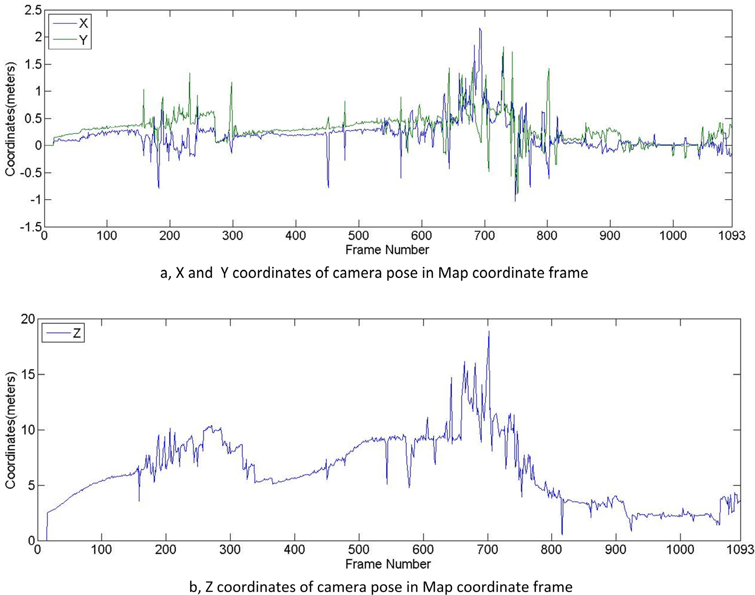
3D pose estimation of the camera in a map coordinate frame

7.4. 3D pose estimation and real-time evaluation

The map in our method is constructed with the feature points found on the vehicle rear. The relative camera poses towards the vehicle rear are the coordinates of the camera in terms of the map coordinates. As shown in Fig. 11, the origin of the map coordinate is the centre of the extracted vehicle rear. The map coordinate is defined in such a way that the X axis and the Y axis are on vehicle rear plane while the Z axis is perpendicular to the vehicle rear plane. Therefore, the measured X and Y values describe the offset of the camera from the origin of the map, namely the centre of the vehicle rear, and the measured Z value is the vertical distance between the camera and the map, namely the vehicle rear. Using the same video clip as that used in section 7.3, the X and Y coordinates of the camera are shown frame-by-frame in Fig. 13(a), while the updating distance between the camera and the map are shown in Fig. 13(b). From Fig. 13(b), we can see the track of these two cars: the two cars were close to each other at the beginning and moved away until the distance reached 18.5 m, and then that the two cars moved closer again and finally stopped when the distance between them was 3.5 m. To demonstrate the performance of our method, we used AR techniques that are strictly dependent on accurate 3D pose estimation in real-time. We used the same 3D model as that in [27]: 3D eyeball models are placed on the origin of the map. As shown in Fig. 14, the changing size of the eyeball models indicates the updating distance between the camera and the map. The changing direction of the eyeball models represents the varying offset between the camera and the origin of the map. We can see that within the entire 1093 frames the 3D models were added on to the accurate position.

Figure 14.

3D model added into the frame based on the estimated pose

Figure 15.

Real-time evaluation

Figure 16.

Evaluation of the map optimization

As to the red line in Fig. 15, the average processing time for each frame was 38.707 ms. In particular, the time includes the license plate detection, the features detection, the 3D pose estimation and the map optimization for each frame. From frame 1 to 15, it took round 25 ms for each frame for license plate detection. The map was constructed during frames 15 and 16, where the processing time jumped to above 90 ms per frame. After the map was constructed, the time for license plate detection, 3D pose estimation and map optimization for each frame did not vary substantially. We can observe that the figure shape of the processing time was similar to that of the feature detection in Fig. 12, where it can be seen that the feature detection primarily accounted for the variation in the processing time.

A demo video can be watched via

http://www.youtube.com/watch?v=m5z5TBsTKwI.

7.5. Evaluation of the map optimization

As explained above, the map is extremely important for accurate pose estimation. It would be highly risky to insert incorrect information into a map as it may expand when new keyframes are found. In order to demonstrate the superiorities flowing from our map optimization method, we tested the proposed method both with and without bundle adjustment optimization on the aforementioned video. As shown in Fig. 16, the red line and the green line denote the keyframe size and the map size with map optimization and frames, respectively. Both of the lines were described in section 7.3: the map size increased when the new keyframes were discovered. Additionally, the map size might decrease when no new keyframe was yielded because some of the outliers were filtered out by bundle adjustment optimization from the set of map points, as the examples show around frames 900 to 1093. On the other hand, the back line represents the evolving map size and the proposed method without map optimization. As can be seen, the map size increased from 158 to 421 map points steadily, along with added keyframes. Furthermore, the black line remained flat when no additional keyframe was found. In this case, errors were prone to occur in pose estimation. In order to put this point into perspective, we still demonstrated the estimated pose by adding the AR model into the video. Fig. 17 gives an example of wrong pose estimation by the proposed method without map optimization: the AR model added in the wrong place, which should have been the front vehicle rear.

7.6. Discussion on lost tracking

The proposed method consists of two threads: tracking and mapping. The importance of accurate map construction and map optimization will be discussed in the last section. This section evaluates the tracking thread of the proposed method. Tracking in our method includes LP tracking and features detection. Lost tracking happens when the LP cannot be found or else when less than 4 features are detected. These botherations are caused by the camera's being far away from the front vehicle, vehicle turning and occlusion. Our system is tolerant of temporary lost tracking, where the map and estimated pose can be kept up for a period. In our experiment, the tolerance of lost tracking is 60 frames. To demonstrate the feasibility of the tolerance setting, we tested the proposed method on the video in which occlusion happened. To make the evaluation comparable, we synthesized a video from the video in Section 7.3 with four temporary occlusions by blocking the ROIs of the frames, which lasted for 50 frames (100 frame—151 frame), 55 frames (200 frame—256 frame), 65 frames (300 frame—366 frame) and 80 frames (400 frame –481 frame). An example of an occluded frame is shown in Fig. 18. Referring to Fig. 19, the red dashed line and the blue dashed line represent the estimated distance and the map on the synthesized video, respectively, while the red line and the blue line plot the estimated distance and the map on the un-occluded video, respectively. When the first and second occlusions happened, the estimated distances (red dashed line) and the map (blue dashed line) remain unchanging, which was acceptable because the distance would not change much over a very short period (around 1 s). After the occlusions end, pose was estimated again with the previous map. When the third and fourth occlusions happened, the distances remained unchanging. However, the map stayed unchanging for the first 60 frames (the set tolerance threshold) while it was initialized again after 60 frames. Pose was then estimated with the newly constructed map after the occlusion ended. Because the map initialization was complemented very quickly (around 15 frames), we observed that the estimated poses (red dashed line) were not affected much in the case of occlusion after comparing it to the one (red line) on the original video.

Figure 17.

An example of wrong pose estimation by the proposed method without map optimization

Figure 18.

In order to make the evaluations comparable, the occluded video is synthesized from the original video

Figure 19.

Evaluation of the method by testing on the original and the synthesized videos

Figure 20.

Stage compliance of method

7.7. Degree of compliance and the method's limitations

As shown in Fig. 20, the proposed method consists of 5 main stages: vehicle rear detection, map initialization, feature detection, mapping and pose estimation. a high degree of compliance on each stage contributes to the final accurate result. Continuing to refer to Fig. 20, the task at each stage should be to complement correctly: 1, the two initial keyframes are detected based on LP detection; 2, the initial stereo algorithm complements correctly, 3, more than 4 features are detected in tracking, 4, the detected features are correctly matched with map points, and 5, the pose estimation algorithm is applied correctly. Though our method is robust at all of these stages, as shown by the experimental analysis above, we experienced two types of failure: the first is a failure in LP localization. Though the effective performance of LP localization was evaluated in section 7.2, the failure of it is indeed a nuisance as it is fundamental to map initialization and tracking. Fortunately, the failure of LP localization always happens when the front vehicle is far away, where the estimate pose of the front vehicle is not especially necessary. The second is a failure of feature detection. This always happen at night. Though the LP can be localized at night because of the existence of vehicle rear lamps, the performance of feature detection is seriously inferior. Therefore, our proposed method is applicable only in daylight.

8. Conclusion

In this paper, we propose a novel visual-based system to estimate the 3D pose of a front vehicle with an onboard camera. Using a combination of line segment features and Haar-like features, the LP is quickly localized. The vehicle rear is extracted based on the localized LP. FAST corners are detected on the vehicle rear. A map containing a set of reference points is initialized from two frames of the extracted vehicle rear at the beginning. After matching the map points with the detected feature points, the relative 3D pose between the current vehicle rear and the camera is calculated frame-by-frame. When new keyframes are found, new feature points would be added into the map. The map is optimized using bundle adjustment when no new keyframe is found. the robustness and accuracy of the proposed method is demonstrated by experimental results. The AR technique is utilized to make the estimated pose in a real-time video visible. With our current method, vehicle rear detection and feature points detection constitute two separate steps. In future work, we intend to find a quicker and more robust method to combine these two steps. Moreover, in order to obtain more accurate and robust pose estimation, an attempt will be made to optimize the process of map initialization and map maintenance.

With our proposed method, the accurate distance of front vehicle can be obtained in real-time. With this information, the driver assistant can alert the driver to reduce their speed and thus avoid collisions when the front vehicle is too close. Furthermore, the future diver assistant can help drivers to make the right decision with a 3D pose estimation of the front vehicle.

Footnotes

9. Acknowledgments

This work is sponsored by the Chinese Scholarship Council (CSC) – Newcastle joint scholarship.

References

B. F.

Juang

J. H.

, “Adaptive Vehicle Detector Approach for Complex Environments,” Intelligent Transportation Systems, IEEE Transactions on, vol. PP, pp. 1–11, 2012.

Vargas

, “An Enhanced Background Estimation Algorithm for Vehicle Detection in Urban Traffic Scenes,” Vehicular Technology, IEEE Transactions on, vol. 59, pp. 3694–3709, 2010.

Papanikolopoulos

N. P.

, “Real-time vehicle following through a novel symmetry-based approach,” in Robotics and Automation, 1997. Proceedings., 1997 IEEE International Conference on, 1997, pp. 3160–3165 vol. 4.

Tzomakas

Seelen

, “Vehicle Detection in Traffic Scenes Using Shadows,” Institutfür Neuroinformatik, Ruht-Universitat, Bochum, Germany, Technical Report98–06 1998.

Betke

, “Real-time multiple vehicle detection and tracking from a moving vehicle,” Machine Vision and Applications, vol. 12, pp. 69–83, 2000.

Cucchiara

, “Image analysis and rule-based reasoning for a traffic monitoring system,” Intelligent Transportation Systems, IEEE Transactions on, vol. 1, pp. 119–130, 2000.

Bucher

, “Image processing and behavior planning for intelligent vehicles,” Industrial Electronics, IEEE Transactions on, vol. 50, pp. 62–75, 2003.

Chu

, “Study on method of detecting preceding vehicle based on monocular camera,” in Intelligent Vehicles Symposium, 2004 IEEE, 2004, pp. 750–755.

Hoffman

, “Vehicle detection fusing 2D visual features,” in Intelligent Vehicles Symposium, 2004 IEEE, 2004, pp. 280–285.

10.

Tai

J.-C.

, “Real-time image tracking for automatic traffic monitoring and enforcement applications,” Image and Vision Computing, vol. 22, pp. 485–501, 2004.

11.

Wei

, “Rear Vehicle Detection and Tracking for Lane Change Assist,” in Intelligent Vehicles Symposium, 2007 IEEE, 2007, pp. 252–257.

12.

O'Malley

, “Rear-Lamp Vehicle Detection and Tracking in Low-Exposure Color Video for Night Conditions,” Intelligent Transportation Systems, IEEE Transactions on, vol. 11, pp. 453–462, 2010.

13.

Raxle

W. Chi-Chen

Lien

J. J. J.

, “Automatic Vehicle Detection Using Local Features—A Statistical Approach,” Intelligent Transportation Systems, IEEE Transactions on, vol. 9, pp. 83–96, 2008.

14.

Negri

, “A Cascade of Boosted Generative and Discriminative Classifiers for Vehicle Detection,” EURASIP Journal on Advances in Signal Processing, vol. 2008, 2008.

15.

Arai

, “Following vehicle detection based on shift of feature plane using affine transform,” in Intelligent Transportation Systems (ITSC), 2010 13th International IEEE Conference on, 2010, pp. 881–886.

16.

Jazayeri

, “Vehicle Detection and Tracking in Car Video Based on Motion Model,” Intelligent Transportation Systems, IEEE Transactions on, vol. 12, pp. 583–595, 2011.

17.

Arrospide

, “Homography-based ground plane detection using a single onboard camera,” Intelligent Transport Systems, IET, vol. 4, pp. 149–160, 2010.

18.

Zielke

“CARTRACK: Computer vision-based car following,” in Applications of Computer Vision, Proceedings, 1992., IEEE Workshop on, 1992, pp. 156–163.

19.

Bensrhair

, “Stereo vision-based feature extraction for vehicle detection,” in Intelligent Vehicle Symposium, 2002. IEEE, 2002, vol. 2, pp. 465–470.

20.

Broggi

, “Obstacle Detection with Stereo Vision for Off-Road Vehicle Navigation,” in Computer Vision and Pattern Recognition - Workshops, 2005. CVPR Workshops. IEEE Computer Society Conference on, 2005, pp. 65–65.

21.

SamYong

, “Front and rear vehicle detection and tracking in the day and night times using vision and sonar sensor fusion,” in Intelligent Robots and Systems, 2005. (IROS 2005). 2005 IEEE/RSJ International Conference on, 2005, pp. 2173–2178.

22.

Zehang

, “A real-time precrash vehicle detection system,” in Applications of Computer Vision, 2002. (WACV 2002). Proceedings. Sixth IEEE Workshop on, 2002, pp. 171–176.

23.

Kawano

, “A coded visual marker for video tracking system based on structured image analysis,” in Mixed and Augmented Reality, 2003. Proceedings. The Second IEEE and ACM International Symposium on, 2003, pp. 262–263.

24.

Eade

Drummond

, “Edge landmarks in monocular SLAM,” Image and Vision Computing, vol. 27, pp. 588–596, 2009.

25.

Mondrago , “3D pose estimation based on planar object tracking for UAVs control,” in Robotics and Automation (ICRA), 2010 IEEE International Conference on, 2010, pp. 35–41.

26.

Mouragnon

, “Real-time Localization and 3D Reconstruction,” in Computer Vision and Pattern Recognition, 2006 IEEE Computer Society Conference on, 2006, pp. 363–370.

27.

Klein

Murray

, “Parallel Tracking and Mapping for Small AR Workspaces,” in Mixed and Augmented Reality, 2007. ISMAR 2007. 6th IEEE and ACM International Symposium on, 2007, pp. 225–234.

28.

Stewénius

, “Recent developments on direct relative orientation,” ISPRS Journal of Photogrammetry and Remote Sensing, vol. 60, pp. 284–294, 2006.

29.

, “Cascade-Based License Plate Localization with Line Segment Features and Haar-Like Features,” in Image and Graphics (ICIG), 2011 Sixth International Conference on, 2011, pp. 1023–1028.

30.

Rosten

Drummond

, “Machine Learning for High-Speed Corner Detection Computer Vision –ECCV 2006.” vol. 3951, Leonardis

, Eds., ed: Springer Berlin / Heidelberg, 2006, pp. 430–443.

31.

Richard

Andrew

, “Multiple View Geometry in Computer Vision,” Cambridge, ISBN 0-521-54051-8. vol. 23, pp. 271–271, 2005.

32.

Huaifeng

, “Learning-Based License Plate Detection Using Global and Local Features,” in Pattern Recognition, 2006. ICPR 2006. 18th International Conference on, 2006, pp. 1102–1105.

33.

Arth

, “Real-Time License Plate Recognition on an Embedded DSP-Platform,” in Computer Vision and Pattern Recognition, 2007. CVPR '07. IEEE Conference on, 2007, pp. 1–8.

34.

Schweighofer

Pinz

, “Robust Pose Estimation from a Planar Target,” Pattern Analysis and Machine Intelligence, IEEE Transactions on, vol. 28, pp. 2024–2030, 2006.

35.

Moré

, “The Levenberg-Marquardt algorithm: Implementation and theory Numerical Analysis.” vol. 630, Watson

, Ed., ed: Springer Berlin / Heidelberg, 1978, pp. 105–116.

Combining Front Vehicle Detection with 3D Pose Estimation for a Better Driver Assistance