Sage Journals: Discover world-class research

Abstract

In this paper we present a new Discrete Particle Swarm Optimization approach to induce rules from discrete data. The proposed algorithm, called Opposition-based Natural Discrete PSO (ONDPSO), initializes its population by taking into account the discrete nature of the data. Particles are encoded using a Natural Encoding scheme. Each member of the population updates its position iteratively on the basis of a newly designed position update rule. Opposition-based learning is implemented in the optimization process. The encoding scheme and position update rule used by the algorithm allows individual terms corresponding to different attributes within the rule's antecedent to be a disjunction of the values of those attributes. The performance of the proposed algorithm is evaluated against seven different datasets using a tenfold testing scheme. The achieved median accuracy is compared against various evolutionary and non-evolutionary classification techniques. The algorithm produces promising results by creating highly accurate and precise rules for each dataset.

Keywords

Particle Swarm Optimization (PSO)Discrete PSO swarm intelligence classification OBL rule list sequential covering algorithm

1. Introduction

Classification is considered one of the most critical tasks of decision-making in a variety of application domains, such as the human sciences, the medical sciences and engineering, etc. Classification schemes have been developed successfully for several applications, such as medical diagnosis, credit scoring and speech recognition, etc. In classification problems, sets of if-then rules for learned hypotheses is considered to be one of the most expressive and comprehensive representations. In many cases, it is useful to learn the target function represented as a set of if-then rules that jointly define the function. There are usually three types of approaches for rule generation using an evolutionary algorithm. In the first approach, an EA evolves a population of rules or a rule baseis evolved by EA such that the whole of the final population or a subset of it is considered to be the end result [1 –6]. The second approach is iterative, running an EA multiple times in succession whereby the result of each run is considered to be a partial solution to the problem [7, 8]. A third approach is to create an ensemble of classifiers by combining several different solutions obtained by using either of the previous two approaches [9 –11].

When considering a rule induction algorithm and focusing on the encoding or representation of rules, there are two main approaches that have been applied by researchers: the Michigan approach and the Pittsburgh approach. If a Michigan-style encoding is applied then, in general, either a rule precondition or a complete rule is evolved by the EA. In the first case, a separate procedure is used to decide the rule postcondition before the rule evaluation, e.g., [1]. Alternatively, the class may already be specified for each rule precondition during the entire run of the algorithm. The EA is run repeatedly with each run focusing on evolving rule preconditions for a specific class, e.g., [12, 13]. If a complete rule is encoded in an individual, then the rule postcondition may also be subject to evolution and change by the genetic operators [2]. In the Pittsburgh approach, rule preconditions are generally encoded along with their postconditions [14].

In this paper, we propose a new Discrete Particle Swarm Optimization technique for discovering classification rules from the given dataset. The salient features of our work are as follows:

We have proposed a new position update rule for the particles with the help of which they can share their information efficiently in a discrete domain.

The proposed position update rule and encoding scheme allows individual terms associated with each attribute in the rule's antecedent to be a disjunction of the values of the attribute. For example, in AM+ [60] and all earlier versions of Ant Miner, the rule antecedent part is simply the conjunction of values of the predicting attributes. In contrast, our technique – ONDPSO – allows a complete rule antecedent to be conjunction of the disjunctions of the values of predicting attributes.

We have introduced a penalty constant in a fitness function of the particles which results in more precise and reliable rules.

The proposed technique works both on binary and multiclass datasets. Although it has been designed for working with datasets containing categorical or discrete attributes, it can also be used in a continuous domain after discretizing the continuous attributes.

This paper is organized as follows. Section 2 describes related work on rule induction using Computational Intelligence techniques. Section 3 provides a brief introduction to classic PSO and its variant, Discrete PSO. Section 4 describes in detail the proposed approach. Next, in Section 5, the experimental setup is discussed and the performance of the proposed algorithm is evaluated on various datasets. Finally, Section 6 concludes with a summary and some ideas for future work.

2. Related Work

Decision trees are one of the most popular choices for rule induction from a given set of training instances. They adapt a divide-and-conquer approach where training data is divided into disjoint subsets and the algorithm is applied to each subset in a recursive manner. First of all, a decision tree is learnt from the data and then it is translated into an equivalent set of rules, one rule for each path from the root to a leaf of the tree [15 –17]. Decision trees tend to suffer from overfitting in the presence of noisy data. Usually some kind of tree-pruning technique is used to get rid of overfitting. Decision trees have been greatly praised for their comprehensibility.

Decision lists are similar to decision trees in that they symbolize an explicit representation of the knowledge extracted from the training data. However, they follow a ‘separate-and-conquer’ approach, where one rule is generated that covers only a subset of the training set and then more rules are built to cover the remaining instances in a recursive manner. This strategy was applied in [18 –20].

Another method applied by researchers for extracting rules from a given dataset is offered by genetic algorithms (GAs). Here, rules are encoded as a bit string and specialized genetic search operators, such as crossover and mutation, are used to explore the hypothesis space, e.g., [4, 21–22]. In [23], a distributed GA-based system, REGAL, has been proposed. It is used to learn first-order logic concept descriptions from training instances. The initial population in REGAL consists of a redundant set of incomplete concept descriptions and each undergoes the evolutionary process separately. G-Net [24] is a robust GA-based classifier that consistently exhibits better performance. Coevolution has been used as a high-level control strategy. G-Net is relatively suitable for parallel implementation on a network of workstations.

Using ant colony optimization (ACO) for rule induction provides an efficient mechanism to accomplish a more global search in a hypothesis space. In [25], an ant algorithm called Ant-Miner was proposed for creating crisp rules for describing the underlying dataset. Ant-Miner considers nodes of a problem graph as the terms that may form a rule precondition. Ant-Miner does not require the ant to visit each and every node. In contrast, [26] takes the rule induction problem as an assignment task where a fixed number of nodes are present in the rule precondition – an ant explores the problem graph by visiting each and every node in turn.

In many classification tasks where Fuzzy systems have been applied successfully, rules are mostly derived from human expert knowledge. However, as the feature space increases, this type of manual approach becomes unfeasible. With this requirement in mind, several methods have been proposed to generate fuzzy rules from numeric data explicitly [27, 28]. The most straightforward fuzzy rule induction methods may be considered as extensions to conventional methods where fuzzy rather than crisp attributes are used. For example, ID3 – a decision tree method – has been extended to produce fuzzy ID3 in the work of [29, 30]. The fuzzy logic-based approach has the major advantage of being able to represent inexact data in a way that is more naturally understood by humans.

Neural networks [31 –35] and GAs [36 –39] have been used by several researchers in combination with fuzzy logic for rule generation.

In [40], genetic programming (GP) using a hybrid Michigan-Pittsburgh-style encoding has been applied to extract rules in an iterative learning fashion. A GP classifier has been proposed in [41], using an artificial immune system-like memory vector to generate multiple comprehensible classification rules. It introduces a concept mapping technique to evaluate the quality of the rules.

Gene Expression Programming (GEP) is a new approach for extracting classification rules by employing genetic programming with linear representation [42]. The antecedent part of the extracted rules may involve many different combinations of the predictor attributes. The search process is guided by a fitness function for the rule quality which takes into account both the completeness and rule consistency. GEP extracts high-order rules for classification problems and a minimum description-length principle is used to avoid overfitting.

In [43], a boosting algorithm has been proposed for learning fuzzy classification rules. An evolution strategy (ES) is iteratively invoked and at each iteration it induces a fuzzy rule that gives the best classification over the current set of training instances. Thus, a rule base is generated in an incremental fashion. The weight of correctly classified training samples is reduced by the boosting mechanism.

The extended classifier system (XCS) represents a major development in learning classifier systems research. XCS [44, 45] has the tendency to evolve classifiers that are as general as possible while still predicting accurately. XCS acts as a reinforcement learning agent with a simplified structure since it does not have an internal message list. The fitness of the classifier is based on the accuracy of the classifier's payoff prediction. XCS uses a modification of Q-learning.

3. Overview of PSO and Discrete PSO

Particle swarm optimization (PSO) is a population-based evolutionary computation technique, originally designed for continuous optimization problems. The searching agents, called “particles”, are ‘flown’ in the n-dimensional search space. Each particle updates its position considering not only its own experience but also that of other particles. The position and velocity of each particle are updated according to the following equations [46]: $X_{i} (t) = X_{i} (t - 1) + V_{i} (t)$ (1) $V_{i} (t) = (w \times V_{i} (t - 1)) + (c_{1} r_{1} (t) (X_{i}^{p b} - X_{i} (t))) + (c_{2} r_{2} (t) (X_{i}^{g b} - X_{i} (t)))$ (2)

where X_i(t) is the position of particle P_i at time t and Vi(t) is the velocity of particle Pi at time t; W is the inertia weight, c1 and c2 are the learning factors; r1 and r2 are constants whose values are randomly chosen between 0 and 1; X_i^pb is the i^th dimension of the personal best position reached so far by the particle under consideration; and X_i^gb is the i^th dimension of the global best position reached so far by the entire swarm. Each particle is evaluated using a fitness function. The closer the position of the particle to the optimal position, the fitter the particle is. The optimization process is iterative.

The PSO algorithm was originally proposed for continuous problems. Kennedy and Eberhart developed the first discrete PSO to operate on binary search spaces [47]. They used the standard velocity update equation but changed the standard position update equation. They considered the new position component to be 1 with a probability acquired by applying a sigmoid function to the corresponding velocity component. This binary PSO is a more specialized version of the general discrete PSO. To obtain a general discrete PSO, the simplest and easiest way is to use standard continuous PSO with the same conventional velocity and position update equation while rounding the elements of the position vectors to the nearest valid discrete value. This approach assumes that elements in the position vector do not take on those values which are outside the extremes of the search space [48, 49]. Another approach is to discretize the continuous space by making intervals and to assign each interval to one of the discrete values [50, 51]. A more sophisticated approach is to redefine the standard arithmetic operators used in position and velocity equations so that they are more suitable for applying to discrete space. For example, in [52], PSO was adapted to be applicable to the constraint satisfaction problem (CSP) by overloading the arithmetic operators used in position and velocity update equations. As such, and in this case, particles represent positions with dimensions that are independent of one another, whereby the changed position and velocity equations are: $X_{i} (t) = X_{i} (t - 1) \oplus V_{i} (t)$ (3) $V_{i} (t) = (w \otimes V_{i} (t - 1)) \circ (c_{1} r_{1} (t) (X_{i}^{p b} Θ X_{i} (t))) \circ (c_{2} r_{2} (t) (X_{i}^{g b} Θ X_{i} (t)))$ (4)

where ⊗, ○, ⊝ and ⊕ are redefined arithmetic operators. Moreover, in [52], a mutation operator was also used which changes each element of the velocity vector based on a certain probability. Similarly, in [53], arithmetic operators were redefined to develop a discrete PSO to solve the travelling salesman problem (TSP). Here, particles represent permutations.

H. R. Tizhoosh first proposed the idea of opposition-based learning (OBL). Suppose we have a real number n within an interval of [a, b], then its opposite number called n' can be calculated as: $n^{'} = a + b - n$ (5)

In order to extend the case to higher dimensions, suppose we have a point N = (n₁,n₂,…,n_m) in an m-dimensional space where n₁, n₂,…,n_m are real numbers and, for each dimension i of N, n_i lies in an interval [a_i, b_i]. The opposite point N = (n₁',n'₂,…,n'_m) is defined by its components: ${n^{'}}_{i} = a_{i} + b_{i} - n_{i}$ (6)

Thus, when implementing opposition-based optimization rather than just evaluating the individuals in an actual population, we compute the opposite individuals as well. If the fitness of an individual is less than the fitness of the corresponding opposite individual, we replace the individual with its counterpart OBL has been implemented successfully in evolutionary algorithms such as DE and PSO to solve different optimization problems.

4. Proposed Method

Suppose that the total number of examples to be classified is N, each of which has M attributes (excluding the class attribute), and that we have a fixed swarm size of P particles. In our proposed algorithm, each particle represents the precondition of an individual rule.

4.1 Particle Encoding and Calculating Opposite Points

The particles have been encoded using Natural Encoding. The position vector of each particle is a string of M natural numbers. In the binary encoding, if m_i is the number of possible values for the i^th attribute, exactly m_i bits are used to encode a value for that attribute. For example, we have an attribute Rain which can take any of the three values Heavy, Medium or Low. We use a bit string of length 3 to encode this attribute. Each bit position in the string corresponds to one of the three values of the attribute Rain. Placing a 1 at a certain position shows that the attribute is allowed to take on the associated value. For example, the string 010 means that Rain takes the second of its three values or (Rain = Medium). Likewise, string 011 means (Rain = Medium or Low). The string 111 represents the most general case, namely that we do not care which of its possible values Rain takes on. Natural encoding for an attribute is obtained by converting a binary number (obtained during its binary encoding) into a natural number [54].

Eq. 6 is used to calculate the opposite point in a continuous space. It cannot be used in a discrete domain. To implement OBL in discrete domain as well, we have used the following equation. More precisely, suppose that Y = (p₁, p₂,…,p_d) is a point in a d dimensional space, then its opposite point Y' = (p'₁, p'₂,…,p'_d) can be calculated as follows: ${p^{'}}_{i} = (2^{k} - 1) - p_{i}$ (7)

where k is the number of unique values for the i^thdimension.

We have explicitly avoided the most specific case (represented by 0 in natural encoding) by not allowing particles to have such Null values. Alternatively, we can simply assign a very low fitness to the particles having such Null values.

4.2 Swarm Initialization

Since swarms learn rules iteratively in a class by class fashion, we have initialized the swarm with the examples of the target class. If the number of examples in the target class is less than the swarm size, the remaining particles are initialized randomly.

4.3 Position Update

We have designed a new position update rule for ONDPSO. The crossover operator used in HIDER* [54] for discrete attributes has been used in our position update rule for both discrete and continuous domains (continuous features are discretized in the pre-processing step). More precisely, the crossover operator works as follows: let n be a natural number, then the natural mutation of the i^th bit of n denoted by mut_j(n) is calculated as: $m u t_{j} = (n + 2^{j - 1}) % 2^{j} + 2^{j} ⌊ \frac{n}{2^{j}} ⌋, k = 1, 2, 3, …, N$ (8)

where N is the number of values of the attribute.

The mutation set Mut(n) is the set of all valid mutations for n. Let t ≥ 0, then the crossover between two natural numbers n_i and n_j is expressed as follows: $C r o s s (n_{i}, n_{j}) = {Z \in Q^{t} | \forall s \geq 0, s < t, Q^{t} \neq \emptyset, Q^{s} = \emptyset}$ (9)

where: $Q^{t} = {[M u t (n_{i})]}^{t} \cap {[M u t (n_{j})]}^{t}$

and: ${[M u t (n_{i})]}^{t} = {\begin{matrix} \underset{n \in {[M u t (n_{i)}]}^{t - 1}}{U} & \begin{matrix} n_{i} i f t = 0 \\ (n \cup M u t (n_{i})) otherwise \end{matrix} \end{matrix}$

In our proposed method, the position of each particle is updated according to the following equation: $X_{i} (t + 1) = C r o s s (C r o s s (X_{i}^{p b}, X_{i} (t)), C r o s s (X_{i}^{g b}, X_{i} (t)))$ (10)

4.4 Quality Measure

In many papers – e.g., [55 –57] – the following fitness function or quality measure has been used to evaluate the performance of a rule: $Q u a l i t y = S e n s i t i v i t y * S p e c i f i c i t y$

“Sensitivity” indicates, out of all positive examples, what ratio of examples is actually classified as positive by the rule, namely: $S e n s i t i v i t y = \frac{t p}{(t p + f n)}$

where tp is the total number of positive examples which are classified as positive by the rule and fn is the total number of positive examples which are not classified as positive by the rule.

“Specificity” indicates, out of all negative examples, what ratio of examples is actually avoided by the rule to be classified as positive, that is: $S p e c i f i c i t y = \frac{t n}{(t n + f p)}$

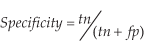
where tn is the total number of negative examples which are not classified as positive by the rule and fp is the total number of negative examples which are classified as positive by the rule.

However, in [58], Nicholas and Alex have shown a scenario where, instead of specificity, precision is more important for assessing the quality of a rule. “Precision” indicates, out of all examples classified as positive by the rule, what ratio of examples is actually positive. It gives us the confidence or reliability of the rule: $\Pr e c i s i o n = \frac{t p}{(t p + f p)}$

Accordingly, Nicholas and Alex replaced “Specificity” with “Precision”. Since we want our iterative rule learning algorithm to be highly precise and since we are ready to accept low coverage, we used a slightly modified version of the quality measure proposed in [48].

The following fitness function or quality measure has been used in our proposed algorithm: $Q u a l i t y = \frac{t p}{t p + f n} * \frac{t p}{(t p + (10^{k} * f p))}$ (11)

where k is a constant used to penalize in instances where the classification is false positive; the greater the value of k, the higher the penalty is. We require that any rule learnt at any time should have a high accuracy, but not necessarily high coverage. By “high accuracy”, we mean that the rule should make correct predictions. By “low coverage” we mean that the rule is not required to make predictions for every training example.

4.5 Stopping Criteria

Since the algorithm learns incrementally – i.e., one rule at a time – there are two different types of stopping criteria. For the evolutionary process where the algorithm is used to learn a single rule, the maximum number of generations specified in advance can be used as stopping criteria. Alternatively, the evolutionary process can be stopped when there is no improvement in the global fitness of the swarm. The second type of stopping criteria is for the overall rule learning scheme. The algorithm continues to extract the best rules for the target class until there are no more examples of the target class in the dataset. This process is repeated for every class.

4.6 Rule Extraction over the Training Data

The proposed algorithm is a class-dependent sequential covering algorithm. For each target class, the algorithm is run to the output of the best rule that describes the examples of that class until either the maximum number of generations has been reached or else there is no improvement in the global fitness of the swarm for a certain number of generations. If the rule performance is above a certain threshold, it is added to the final rule list. Otherwise, the threshold is decreased linearly. For each target class, it continues to learn rules sequentially and removes the covered examples of the class until there is no more example of the target class. At this point, dataset is set to the original dataset with all the training examples and the algorithm proceeds to learn rules for another target class.

Negative examples – i.e., those which belong to a class other than the current target class – are also used in the evolutionary process so that classification may be more directed and precise, otherwise the algorithm may end up by returning the single and most general rule for the target class where the encoded string contains all 1's in it.

Presented below is the pseudo-code describing the proposed technique:

For each class, perform steps 2 and 3

reinitialize the training set

while some examples of the class are still uncovered, perform steps 4 to 6

run our discrete PSO to generate the best rule using the position update method described at the end of Section 4.3

if the best rule performance >= the threshold

add the best rule to the final rule set

remove the covered class examples, and

go to step (3)

else decrease the threshold, go to step (4)

output the final rule set

4.7 Classifying Test Data

In applying the final rule list in the test phase, an unseen example has been checked against all the rules in the rule. If none of the rules match the example, it is assigned the default class, which is the majority class in the dataset. If more than one rule matches the example but all the rules predict the same class, then this class will be assigned to the example. If the matching rules are in conflict with each other in predicting the class, then we have adopted the conflict resolution strategy described in [59]. The pseudo-code for this strategy is as under:

For each class c in the dataset, initialize count(c) to zero. For each conflicting rule r For each class c Add to count(c) the number of training cases with class c covered by rule r End for End for

The unsigned example will be assigned to the class c, which has the highest count(c) among all the classes.

5. Experiments and Results

5.1 Datasets & Experimental Setup

Seven datasets have been used in our experiments. The datasets have been downloaded from the online UCI Machine Learning Repository [61]. The information about these datasets has been summarized in Table 1. We have used a population size of 40 in all the experiments unless stated otherwise. The threshold is initially set to 0.25. The algorithm is given a chance to find the rule whose quality is greater than or equal to the threshold. If it fails to do so, the threshold is decreased by multiplying it with a scaling factor. The scaling factor is set to 0.7. During the phase of learning a single rule, we have allowed the algorithm to run for a maximum of 1,000 generations. The threshold for early stopping is set to 5% – i.e., the algorithm continues to extract rules for the target class until 5% of the examples of the target class remain uncovered. Continuous attributes, when present in the dataset, have been discretized in the pre-processing step using Weka's supervised discretization method. In each experiment, we have used a ten-folding testing scheme. We have defined “error” to be the sum of the fp and fn. This experimental set up is summarized in Table 2.

Table 1.

Datasets Used in Experiments

Dataset	No. of Continuous Attributes	No. of Discrete Attributes	No. of Classes
Lenses	0	4	3
Zoo	0	16	7
Mushroom	0	22	2
Pima Indian	8	0	2
Iris	4	0	3
Wine	13	0	3
Breast	9	0	2

Table 2.

Experimental Setup

Population	40
Max No. of Iterations	1000
Performance Threshold	0.25
Scaling Factor for Threshold	0.7
Early stopping	5%
K	6
Testing Scheme	10-fold

5.2 Results

5.2.1 Initialization

Usually, all the particles in the swarm are initialized randomly. We have initialized the particles with examples of the target class as well so as to observe the effects on accuracy, T/R (the term to rule ratio), R (the number of rules in the final rule list) and FE (fitness evaluations). The results showed that random initialization exhibited relatively poor performance as compared to the alternative initialization scheme. As shown in Figure 1, initialization with the target examples exhibited greater accuracy than random initialization on 3 out of 4 datasets. On the lenses dataset, both initialization schemes resulted in the same accuracy. Similarly, Figure 2 and Figure 3 show that initialization with target examples achieved a lower median value for T/R and R for the four datasets, except for lenses where both schemes performed equally well.

Figure 1.

Comparing Percentage Accuracy

Figure 2.

Comparing T/R

Figure 3.

Comparing No. of Rules

Figure 4.

Comparing FE

5.2.2 Pruning

We have also experimented to observe the effects of pruning and to see what difference it brings to the T/R, R and accuracy statistics. Figure 5 shows the comparison of the percentage median accuracy achieved by pruning and without pruning the rules. It is very clear that pruning always resulted in better percentage median accuracy in all cases. The difference is significant for wine and zoo datasets where the pruning succeeded in achieving 100% accuracy. By using pruning, we mainly hoped to achieve a lower value for T/R. Figure 6 shows that the results are in complete accordance with our viewpoint. Pruning the rules resulted in a lower T/R for all the datasets. Again, the results are more significant for the wine and zoo datasets where the reduction of the T/R value is more than 66%. These results also confirm the viewpoint that shorter or more general rules result in better accuracy for a given dataset. Figure 7 shows the comparison between numbers of rules in the final rule list. Figure 8 shows that in most of the cases there was no effect on the number of FE.

Figure 5.

Comparing Percentage Accuracy

Figure 6.

Comparing T/R

Figure 7.

Comparing No. of Rules

Figure 8.

Comparing FE

5.2.3 Conflict Resolution

We have also experimented to see the effects of applying a final rule list in different ways in the testing phase. In one case, the final rule list is sorted according to the rule quality in descending order before the start of testing. A class is assigned to the unseen example on the basis of which rule first matches the example. As an alternative, we did not sort the final rule list and an unseen example was checked against all the rules in the rule list. In cases where more than one rule matches the example, a conflict resolution strategy has been used to resolve the conflict as described in Section 4.7. Figure 9 shows that better percentage median accuracy has been achieved by conflict resolution scheme when compared to the sorted rule list scheme.

Figure 9.

Comparing Percentage Accuracy

5.2.4 Performance of ONDPSO and its Comparison with Other Techniques

We have compared the performance of our approach over the seven datasets listed in Table 1 with the results reported in [54]. The experimental set up described in Table 2 has been used along with the pruning mechanism. Moreover, the conflict resolution strategy was used in the testing phase. The performance statistics of ONDPSO in terms of average percentage error, number of rules R, terms to rule ratio T/R and number of fitness evaluations FE are reported in Table 3.

Table 3.

Performance of ONDPSO over Different Datasets

Datasets	% Median Error	Median R	Median T/R	Median FE
Iris	3.30	9.00	1.60	1920000
Wine	0.00	6.50	2.50	33280
Lenses	0.00	4.00	2.50	16620
Zoo	0.00	9.00	2.40	33460
PimaIndian	33.76	30.00	3.42	6822200
Mushroom	1.60	9.00	2.05	72280
Bcw	2.86	11.00	4.02	130240

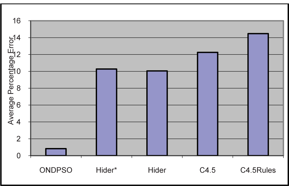
Table 4 shows the results where, for the seven datasets, the obtained percentage median accuracy achieved by ONDPSO has been compared with the results reported in [54]. As shown in Table 4, our proposed algorithm ONDPSO exhibited better performance in terms of error rate when compared with other techniques. On the iris dataset, ONDPSO performed better than the C4.5 and C4.5 rules but stood equal to Hider and Hider*. In case of the breast cancer dataset, ONDPSO achieved a smaller error rate than all the other techniques but the difference is especially larger in case of C4.5. ONDPSO performed significantly well on the wine, lenses and zoo datasets and left the other 4 techniques behind. More importantly, it succeeded in achieving a 0% error rate in the case of these three datasets. Pima Indian and mushroom are the two datasets where ONDPSO performed poorly when compared to the other techniques.

Table 4.

Comparison of the Error Rate (ER) and Number of Rules (NR)

Datasets		ONDPSO		Hider		Hider*		C4.5		C4.5 Rules
Datasets		ER	NR	ER	NR	ER	NR	ER	NR	ER	NR
Multiclass	Iris	3.30	9.00	3.30	4.80	3.30	3.20	5.30	5.70	4.70	5.00
	Wine	0.00	6.50	3.90	3.30	8.80	5.60	6.70	6.50	6.70	5.60
	Lenses	0.00	4.00	25.00	6.50	25.00	4.50	30.00	5.20	16.70	4.10
	Zoo	0.00	9.00	8.00	7.20	4.00	7.90	7.00	10.90	29.80	6.30
Binary	Pima Indian	33.76	30.00	25.90	16.60	25.70	5.10	26.10	24.40	29.70	8.30
	Mushroom	1.60	9.00	0.80	3.10	1.20	3.50	0.00	17.60	0.70	17.90
	Bcw	2.86	11.00	4.30	2.60	4.10	2.00	6.30	22.90	4.90	9.60

Figure 10 clearly shows that, most of the time during the testing phase, the algorithm stayed closer to its best performance – i.e., a low error rate. Figure 11 and Figure 12 show the performance of ONDPSO and the other techniques on multiclass and binary datasets respectively.

Figure 10.

Min, Median and Max. Error by ONDPSO

Figure 11.

Average Percentage Error Over Multiclass Datasets

Figure 12.

Average Percentage Error Over Binary Datasets

Overall, when the percentage error rate was averaged over all the datasets, ONDPSO achieved the lowest error rate of 6.04%. Hider and Hider* stayed very close to each other. C4.5 produced the highest error rate at 13.31%. These results are shown in Figure 13.

Figure 13.

Overall Average Percentage Error

However, as far as the number of rules or the size of extracted rule list is concerned, ONDPSO produced a comparatively longer rule list when compared with the Hider, Hider* and C4.5 rules. The difference is especially significant on the iris and breast cancer datasets whereas on the remaining 3 datasets, ONDPSO stayed very close to HIDER* and produced nearly equally-sized rule lists. Only in comparison with C4.5 did ONDPSO extract shorter rule lists on average.

Having chosen the natural encoding for the particles, our newly designed position update rule exhibited better performance statistics when compared to the results reported in [54, 60]. Together with the position update rule, the chosen quality measure helped the algorithm in extracting very precise rules, with each rule having comparatively less coverage. As a result of this, ONDPSO produced higher accuracy statistics and longer rule lists for each dataset.

6. Conclusion

In this paper, we have proposed an algorithm for rule extraction called ONDPSO. The aim of the proposed technique is to discover classification rules in the dataset. Though the algorithm has been designed for working with datasets containing categorical or discrete attributes, it can also be used in continuous domains after discretizing the continuous attributes. It discovers rules where individual terms in the rule's antecedent are allowed to be disjunctions of the possible values of those attributes. We have compared the accuracy of ONDPSO with various evolutionary and non-evolutionary techniques over seven different public domain datasets. As we have shown, ONDPSO achieved 100% accuracy on the wine, zoo and lenses datasets.

In the future, we would be interested in coming up with some modifications that may result in relatively shorter rule lists. We are also interested in finding new position update rule for the particles.

References

Ishibuchi

Nakashima

and Murata

Performance Evaluation of Fuzzy Classifier Systems for Multidimensional Pattern Classification Problems. IEEE Transactions on Systems, Man and Cybernetics 29:601–618, 1999.

Yuan

Y.F.

and Zhuang

A Genetic Algorithm for Generating Fuzzy Classification Rules. Fuzzy Sets and Systems 84:1–19, 1996.

Slawinski

Krone

Hammel

Wiesmann

and Krause

A Hybrid Evolutionary Search Concept for Data-Based Generation of Relevant Fuzzy Rules in High Dimensional Spaces. Proceedings of the IEEE International Conference on Fuzzy Systems (FUZZ IEEE 1999) 3:1432–1437, 1999.

de Jong

K. A.

Spears

W. M.

and Gordon

D.F.

Using Genetic Algorithms for Concept Learning. Machine Learning 13:161–188, 1993.

Janikow

C.Z.

A Knowledge-Intensive Genetic Algorithm for Supervised Learning. Machine Learning 13:189–228, 1993.

Ishibuchi

Nakashima

and Murata

Genetic-Algorithm-Based Approaches to the Design of Fuzzy Systems for Multi-Dimensional Pattern Classification Problems. 229–234, 1996.

Riquelme

J. C.

Aguilar

J.S.

and Toro

Discovering Hierarchical Decision Rules with Evolutive Algorithms in Supervised Learning. International Journal of Computers, Systems and Signals 1:73–84, 2000.

Liu

J. J.

and Kwok

J.T.

An Extended Genetic Rule Induction Algorithm. Proceedings of the 2000 Congress on Evolutionary Computation (CEC-2000) 458–463, 2000.

Sirlantzis

Fairhurst

M.C.

and Guest

R.M.

An Evolutionary Algorithm for Classifier and Combination Rule Selection in Multiple Classifier Systems. Proceedings of the International Conference on Pattern Recognition 2:771–774, 2002.

10.

Langdon

W. B.

and Buxton

B.F.

Genetic Programming for Combining Classifiers. Proceedings of the Genetic and Evolutionary Computation Conference (GECCO-2001)

11.

Kim

Street

W.N.

and Menczer

Meta-Evolutionary Ensembles. Proceedings of the IEEE International Joint Conference on Neural Networks (IJCNN 2002) 2791–2796, 2002.

12.

Gonzalez

and Perez

Completeness and Consistency Conditions for Learning Fuzzy Rules. Fuzzy Sets and Systems 96:37–51, 1998.

13.

Romao

Freitas

A.A.

and Pacheco

R.C.S.

A Genetic Algorithm for Discovering Interesting Fuzzy Prediction Rules: Applications to Science and Technology Data. Proceedings of the Genetic and Evolutionary Computation Conference (GECCO-2002) 343–350, 2002.

14.

Smith

S. F.

A learning system based on genetic adaptive algorithms. Doctoral dissertation, Department of Computer Science. University of Pittsburgh, 1980.

15.

Gallion

St. Clair

D.C.

Sabharwal

and Bond

W.E.

Dynamic ID3: A Symbolic Learning Algorithm for Many-Valued Attribute Domains. Proceedings of the 1993 Symposium on Applied Computing 14–20, 1993.

16.

Quinlan

J. R.

Induction on Decision Trees. Machine Learning 1:81–106, 1986.

17.

Quinlan

J. R.

Decision Trees as Probabilistic Classifiers. Proceedings of the Fourth International Workshop on Machine Learning 31–37, 1987.

18.

Michalski

R. S.

and Chilausky

R.L.

Learning by being told and learning from examples. International Journal of Policy Analysis and Information Systems 4:125–161, 1980.

19.

Clark

and Niblett

The CN2 induction algorithm. Machine Learning 3(4):261–283, 1989.

20.

Rivest

R. L.

Ronald

Learning decision lists. Machine Learning 2:229–246, 1987.

21.

Janikow

C. Z.

A knowledge-intensive GA for supervised learning. Machine Learning 13:189–228, 1993.

22.

Booker

L. B.

Goldberg

D.E.

and Holland

J.H.

Classifier systems and genetic algorithms. Artificial Intelligence 40:235–282, 1989.

23.

Giordana

and Neri

Search-intensive concept induction. Evol. Comput. 3(4):375–416, 1995.

24.

Anglano

and Botta

NOW G-Net: Learning classification programs on networks of workstations. IEEE Trans. Evol. Comput. 6(5):463–480, Oct. 2002.

25.

Parpinelli

R. S.

Lopes

H.S.

and Freitas

A.A.

Data Mining with an Ant Colony Optimization Algorithm. IEEE Transactions on Evolutionary Computation 6:321–332, 2002.

26.

Casillas

Cordon

and Herrera

Learning Fuzzy Rules using Ant Colony Optimization Algorithms. Proceedings of the 2nd International Workshop on Ant Algorithms (ANTS 2000) 13–21, 2000.

27.

Abe

and Lan

Fuzzy rules extraction directly from numerical data for function approximation. IEEE Transactions on Systems, Man and Cybernetics, 25(1):119–129, 1995.

28.

Delagado

Gomez-Skorneta

A.F.

and Martin

A fuzzy clustering-based rapid prototyping for fuzzy rule-based modelling. IEEE Transactions on Fuzzy Systems 5(2):223–233, 1997.

29.

Umano

Okamoto

Hatono

and Tamura

Generation of fuzzy decision trees by fuzzy id3 algorithm and its application to diagnosis by gas in oil, Japan-U.S.A. Symposium, pp. 1445–1450, 1994.

30.

Janikow

C. Z.

Learning Fuzzy Controllers by Genetic Algorithms. Proceedings of the 1994 ACM Symposium on Applied Computing 232–236, 1994.

31.

Yao

Wei

and He

Evolving fuzzy neural networks for extracting rules. Proc. 5th IEEE Int. Conf. Fuzzy Systems (FUZZ-IEEE '96) 361–367, 1996.

32.

Lee

Kwang

and Wang

L.H.

A fuzzy neural network model for fuzzy inference and rule tuning. Int. J. Uncertainty, Fuzziness Knowledge- Based Syst. 2:265–277, 1994.

33.

Ishibuchi

Fujioka

and Tanaka

Neural networks that learn from fuzzy if-then rules. IEEE Trans. Fuzzy Syst. 1:85–97, 1993.

34.

Pal

N. R.

and Pal

On rule pruning using fuzzy neural networks. Fuzzy Sets Syst. 106:335–347, 1999.

35.

Shann

J. J.

and Fu

H.C.

A fuzzy neural network for rule acquiring on fuzzy control system. Fuzzy Sets Syst. 71:345–357, 1995.

36.

Pal

Evolutionary approaches to rule extraction for fuzzy logic controllers. Advances in Soft Computing, (Lecture Notes Series in Artificial Intelligence) 2275: 425–432, 2002.

37.

Roubos

B. H.

and Setnes

Compact fuzzy models through complexity reduction and evolutionary optimization. Proc. 9th IEEE Int. Conf. Fuzzy Systems (FUZZ-IEEE'2000) 2:762–767, 2000.

38.

Krone

Krause

and Slawinski

A new rule reduction method for finding interpretable and small rule bases in high dimensional search spaces. Proc. 9th IEEE Int. Conf. Fuzzy Systems (FUZZ-IEEE'2000) 2:694–699, 2000.

39.

Chan

P. T.

Xie

W.F.

and Rad

A.B.

Tuning of fuzzy controller for an open-loop unstable system: A genetic approach. Fuzzy Sets Syst. 111:137–152, 2000.

40.

Mendes

R. R. F.

Voznika

F.d.B.

Freitas

A.A.

and Nievola

J.C.

Discovering Fuzzy Classification Rules with Genetic Programming and Co-Evolution. Lecture Notes in Artificial Intelligence 2168:314–325, 2001.

41.

Tan

K. C.

Tay

Lee

T.H.

and Heng

C.M.

Mining Multiple Comprehensible Classification Rules using Genetic Programming. Proceedings of the Congress on Evolutionary Computation. CEC '02., 2:1302–1307, 2002.

42.

Zhou

Xiao

Tirpak

T.M.

and Nelson

P.C.

Evolving accurate and compact classification rules with gene expression programming. IEEE Trans. Evol. Comput. 7(6):519–531, Dec. 2003.

43.

Hoffmann

Combining Boosting and Evolutionary Algorithms for Learning of Fuzzy Classification Rules. Fuzzy Sets and Systems, Article in Press – Uncorrected Proof, 2003.

44.

Wilson

S. W.

Classifier fitness based on accuracy. Evol. Comput. 3(2):149–175, 1995.

45.

Butz

M. V.

Kovacs

Lanzi

P.L.

and Wilson

S.W.

Toward a theory of generalization and learning in XCS. IEEE Trans. Evol. Comput. 8(1):28–46, Feb. 2004.

46.

Kennedy

and Eberhart

R.C.

Particle swarm optimization. Proc. IEEE Int. Conf. Neural Networks 1942–1948, 1995.

47.

Kennedy

and Eberhart

R.C.

A Discrete Binary Version of the Particle Swarm Algorithm. Proceedings of the World Multiconferenceon Systemics, Cybernetics and Informatics 4104–4109, 1997.

48.

Laskari

E. C.

Parsopoulos

K.E.

and Vrahatis

M.N.

Particle Swarm Optimization for Integer programming. Proceedings of the IEEE Congress on Evolutionary Computation 2:1582–1587, 2002.

49.

Salman

Ahmad

and Ai-Madani

Particle Swarm Optimization for Task Assignment Problem. Microprocessors and Microsystems 26(8):363–371, 2002.

50.

Yoshida

Kawata

Fukuyama

and Nakanishi

A Particle Swarm Optimization for Reactive Power and Voltage Control Considering Voltage Stability. Proceedings of the International Conference on Intelligent System Application to Power System 117–121, 1999.

51.

Fukuyama

Takayama

Nakanishi

and Yoshida

A Particle Swarm Optimization for Reactive Power and Voltage Control in Electric Power Systems. Proceedings of the Genetic and Evolutionary Computation Conference 1523–1528, 1999.

52.

Schoofs

and Naudts

Swarm Intelligence on the Binary Constraint Satisfaction Problem. Proceedings of the IEEE Congress on Evolutionary Computation 2:1444–1449, 2002.

53.

Clerc

Discrete Particle Swarm Optimization Illustrated by the Traveling Salesman Problem. Technical report, 2000, http://clerc.mauriceJree.fr/pso/

54.

Aguilar-Ruiz

Giráldez

and Cristóbal

Natural Encoding for Evolutionary Supervised Learning. IEEE Transactions on Evolutionary Computation 11(4):466–479, 2007.

55.

Alves

R.T.

Delgado

M.R.

Lopes

H.S.

and Freitas

A.A.

An artificial immune system for fuzzy-rule induction in data mining. Proc. Parallel Problem Solving from Nature (PPSN-2004), LNCS 3242:1011–1020, 2004.

56.

Sousa

Silva

and Neves

Particle Swarm based Data Mining Algorithms for classification tasks. Parallel Computing 30:767–783, 2004.

57.

Parpinelli

R. S.

Lopes

H.S.

and Freitas

A.A.

Data Mining with an Ant Colony Optimization Algorithm. IEEE Trans. on Evolutionary Computation, special issue on Ant Colony algorithms 6(4):321–332, 2002.

58.

Holden

and Freitas

A.A.

Hierarchical classification of G-Protein-coupled receptors with a PSO/ACO algorithm. Proc. IEEE Swarm Intelligence Symposium 77–84, 2006.

59.

Smaldon

Freitas

A.A.

A New Version of the Ant-Miner Algorithm Discovering Unordered Rule Sets. In Proceedings of the Genetic and Evolutionary Computation Conference (GECCO-2006), 43–50.

60.

Martens

and Baker

M.D.

Classification with ant colony optimization. IEEE Transactions on Evolutionary Computation, 11(5):651–665, 2007.

61.

http://archive.ics.uci.edu/ml/