Sage Journals: Discover world-class research

Abstract

This paper describes our work in developing a 3D robotic mapping system composed by an experimental mobile platform equipped with a rotating laser range finder (LRF). For the purpose of obtaining more complete 3D scans of the environment, we design, construct and calibrate a crank-rocker four-bar linkage so that a LRF mounted on it could undergo repetitive rotational motion between two extreme positions, allowing both horizontal and vertical scans. To reduce the complexity of map representation suitable for optimization later, the local map from the LRF is a grid map represented by a distance-transformed (DT) matrix. We compare the DT-transformed maps and find the transformation matrix of a robot pose by a linear simplex-based map optimization method restricted to a local region allows efficient alignment of maps in scan matching. Several indoor 2D and 3D mapping experiments are presented to demonstrate the consistency, efficiency and accuracy of the 3D mapping system for a mobile robot that is stationary or in motion.

Keywords

Slam 3D Mapping Rotating Laser Range Finder

1. Introduction

Building an environment map is a popular topic in mobile robotic research and applications. The method of how to get information on the environment and robot localization is called SLAM (Simultaneous Localization and Mapping) [1 –10]. With uncertainties in the environment and sensor readings, SLAM is one of the most fundamental methods for enhancing the robustness and efficiency of mobile robot navigation [5, 8], path planning, pursuing and patrolling.

Since the range measurements are inaccurate and noisy, the mapping process is error prone. There are two major methods for constructing a map precisely and efficiently. One is a probabilistic method [28] and the other is scan matching. In the probabilistic method, EKF (Extended Kalman Filter) [8, 9] and RBPF (Rao-Blackwell particle filter) [10, 11] have been used in SLAM for a long time. The features [12] of the map are defined by probability and the feature with the highest probability is the true map's information. Because of the advantage of a continuously correct characteristic, the errors in the probabilistic method can be decreased from the correct features. On the other hand, due to the heavy matrix computation time, the method only uses the few features. Scan matching registers (and extracts the similar parts of) two laser scans obtained at pose 1 and pose 2, in order to determine their relative position and orientation, to obtain the pose-to-pose rigid body transformation matrix T (x, y, θ) that will project the points at pose 2 so that they align with pose 1. The method of scan matching is based on comparing all the information and finding the transformation matrix that has the highest overlapping area. This method can be categorized into feature to feature, point to feature and point to point. In the feature to feature approaches, the properties of laser scanned data, such as line segments and corners, are extracted and then matched directly [15, 16]. This kind of approach requires the features' extraction from laser scanned data. In feature approaches the features, such as lines, are extracted from reference scanned data and form a predefined map. Then the current scanned data is matched to this predefined map. The iterative closest point (ICP) algorithm is the most popular method for aligning two different point sets in 2D scan matching [14] or 3D mapping [13], [31]. In the ICP method, the total squared distance between the points in the current scan and the corresponding points in the reference scan is iteratively minimized for the registration of point clouds.

For a robotic mapping task, the preferred sensor is a laser range finder (LRF). However, a 2D scanner mounted on the robot takes measurements in the horizontal plane only and thus only a 2D map can be built. For autonomous and safe navigation for long periods of time, it is necessary to provide a robot with 3D environment information, such as objects and ceiling, rather than a 2D map. For approaches to 3D mapping and 3D shape sensing, [28] used two LRFs, one horizontal and one vertical, to generate accurate 3D maps by registering the horizontal scans. One cost-effective approach to extend the 2D map to the 3D map that we adopt in this paper is to rotate a LRF to acquire 3D data on the environment by designing an actuated rotating mechanism [18 –23, 29 –31], while the horizontal scans are used to estimate the robot pose. Figure 1 shows conceptually how to expand the 2D map to a 3D map by rotating a LRF with a different elevation and a cloud of 3D data is obtained by combining the 2D data with the elevation information. The motion of a rotating LRF can be defined by two methods: continuing [22] or reciprocation [23]. There are three rotational directions for an actuated LRF using different rotational mechanism designs for 3D mapping robots [19 –21, 29 –31], which yield different scanning ranges (as depicted in Figure 2) and thus different functionality in 3D mapping tasks.

Figure 1.

An LRF is rotated to obtain the 3D mapping data at different elevation of its covered area.

Figure 2.

Different motions on the actuated LRF yield different sensing information [18].

This paper presents the development of an actuated LRF-based robotic 3D indoor mapping system based on transforming the scanning data of a LRF into a distance transform (DT) map for a scan matcher. DT maps are then used to compare the contrasting robot poses defined by a transformation matrix T(x, y, θ). A linear simplex optimization method [17] is applied to find a transformation matrix T* that yields maximum overlap between two maps.

T* defines the robot localization. We design a crank-rocker four-bar linkage to rotate the LRF mounted on it, so that the LRF can scan both horizontally and vertically to continuously acquire 3D mapping data when the mobile robot is stationary or in motion. A composite transformation is derived to transform the 2D data of the LRF to 3D data in the global map, which is set as the map in the first scan.

The organization of the paper is as follows. Section 2 presents the 2D mapping system with the specific mobile platform for experiments. Section 3 presents the details of our crank-rocker design and its integrated use in 3D mapping systems with demonstrated experimental results showing the usefulness of the mapping system. Conclusions are made in Section 4.

2. 2D mapping

2.1 Preliminaries

2.1.1 DT (Distance Transform)

The distance transformation (DT) [27] provides each grid of a grid map with the Euclidean distance to the nearest obstacle. The DT transforms the information from an LRF into a matrix Each element of the matrix stands for the distance to the nearest obstacle on the map In this paper, we use the Euclidean distance transformation as the DT algorithm in (1)

$DT(x, y) = \min {{(x - i)}^{2} + {(y - j)}^{2} : i = 1, ..., M \land j = 1, ..., N}$ (1)

where M and N are the size of DT Figure 3 illustrates a map before (a) and after (b) DT Figure 5 shows the raw scanned map from an LRF and its intensity map after DT The intensity map has the contours of the original map.

Figure 3.

(a) The map before DT. The value of grids that obstacle occupies is initially set to zero and other positions are set to infinity. (b) The map after DT. The distance to the closest obstacle is set as the grid value of every non-obstacle position.

Figure 4.

(a) The map from LRF. (b) The intensity map after DT.

Figure 5.

The flow chart of 2D mapping system based on scan matching

2.1.2 Transformation matrix

The 2D transformation matrix between two consecutive maps is composed of a translation (xy) and a rotation specified by an angles defined as

$T (x, y, θ) = [\begin{matrix} \cos θ & - \sin θ & x \\ \sin θ & \cos θ & y \\ 0 & 0 & 1 \end{matrix}]$ (2)

For a collection of maps at different time steps{P(t+i), i=0,…, n}, the transformation matrix from time t to t+n can be found by simply multiplying the transformation between two consecutive maps as:

$T_{t}^{t + n} = T_{t}^{t + 1} \cdot T_{t + 1}^{t + 2} \dots T_{t + n - 1}^{t + n} = T_{t}^{t + n - 1} \cdot T_{t + n - 1}^{t + n}$ (3)

where each T is of the form (2).

There are many sources of error when two maps are matched with each other. Scan matching is used to find a T_t^t+n value to align the comparative maps with maximum overlap so that the new map from the LRF scan highly coincides with the comparative map. The optimal transformation matrix T_t^t⁺ⁿ at time n is obtained as a result of the minimization of a cost function defined as the sum of the distances to the obstacles of this map:

$\underset{T_{t}^{t + n}}{\arg} \min \sum_{i = 1}^{m} D T (T_{t}^{t + n} \cdot P_{i})$ (4)

where P_i =(P_x, P_y 1) is the point of the obstacles.

2.2 2D mapping systems

In the method of scan matching, it is necessary to predict the position of the robot as an initial guess and thus predict the map, which has new information that the global map doesn't have. A correct prediction can be used to speed up the SLAM process and build a more accurate map. Figure 5 shows our approach to 2D SLAM (cf. [34]), which is extended to 3D mapping in the next section. It consists of the different steps during the mapping processes. First, our implementation uses the information from motor encoders for the transformation matrix of a robot pose to predict the LRF data on the global position, while the LRF acquires the 2D information of the environment. In step 2, the data from the LRF is transformed to a DT matrix as a representation of the local map to be compared with the robot's localization. The optimization method is exploited to solve (4) and to find the optimal transformation matrix that yields maximum overlap. In step 3, the transformation matrix obtained in step 2 is used to construct the environment map using Global Distance Transform (GDT) definition (Sec. 2.4) to combine the global map's DT and the new map's DT.

2.3 Kinetic formula of experimental mobile platform

Figure 6(a) shows our experimental mobile platform: a four wheeled robot with two motors on the front wheels. The LRF is mounted on the centre O of the front of the robot and rotated by a four-bar linkage platform on the mobile robot to allow both horizontal and vertical scans. We need to find the relative motion x, y, θ between O_t and O_t+₁ of the centre at time instants t and t + 1, as depicted in Figure 6(b), given the inputs of the speed L_v, Rv, of the left and right driving wheels at time t and the width of the robot W.

Figure 6.

(a)Experimental mobile platform- a four-wheeled robot with two front driving wheels and two supporting wheels (b) The kinetic formula of vehicle motion between two consecutive time instants

At first the distance travelled by wheels Ld, Rd in one time step Δt is given by L_d=L_vΔt, R_d=R_vΔt. The x,y, θ of relative motion between O_t and O_t+1 is given in (5) using the triangular ratio:

$x = W_{0} \cos θ, y = W_{0} \sin θ, θ = {\frac{180 \cdot L_{d}}{π \cdot W_{0}}}_{}$ (5)

where W₀ + W is the turning radius at time t.

Instead of matching two consecutive maps, we set the DT map of the first scan at t=t to be the global distance transformation map (GDT) and the reference map for the scan matcher. In order to register newly scanned maps with GDT through maximum overlap between the maps, a prediction of the position and orientation of the robot is proposed. From the kinetic formula (5), we can get the predicted robot pose TM(x, y, θ) using a motor encoder. Then the predicted position P_pre.of a data point from the LRF is.

$\begin{array}{l} P_{p r e} = (x_{p r e}, y_{p r e}) \\ = T_{M} \cdot P_{} \end{array}$ (6)

Denote DT_pre as DT of P_pre. Then the size Ω of DT_pre is the extreme x, y values of P_pre. and defined in (6), i.e.,

$Ω = [[M i n (x_{p r e}), M a x (x_{p r e})] \times [M i n (y_{p r e}), M a x (y_{p r e})]$

A prediction of the position (i, j) of the map in GDT is obtained as:

$D T_{p r e} = G D T (i, j), (i, j) \in Ω$ (7)

In performing scan matching to find the optimal transformation matrix described in Sec. 2.1.2, those P_pre points with DT values higher than a threshold Δ

${P_{p r e} : D T_{p r e} > Δ}$ (8)

that may cause a faulty match are discarded temporarily to maximize the overlap of the newly scanned map and the global map. After comparing the maps, these eliminated points are added back into the global map with the matched points to complete the prediction of the global map. In our implementation, we set:

$Δ = R_{M} \sin (γ)$

where R_M = 20 m is the maximum range and γ = 0.250 is the angular resolution of the LRF in a scan.

2.4 Global DT definition for update of GDT map

For each newly created DT map obtained from a new scan, its new information is combined to the GDT to update the map. To combine an existing GDT and a new DT as an updated GDT for each scan, we need to compare all the elements in the existing GDT and the newly created DT. There are three different situations when comparing each element (i,j) ∈ Ω (a)GDT(i, j) and DT(i, j) are close enough. Then updated GDT(i, j) is the average of GDT(i, j) and DT(i, j) in (9).

$\begin{array}{l} u p d a t e d G D T (i, j) = \frac{1}{2} (G D T (i, j) + D T (i, j)), \\ i f | G D T (i, j) - D T (i, j | < T h r e s h o l d \end{array}$ (9)

(b)GDT(i, j) is higher than DT(i, j). This point does not add new information of the environment with the existing GDT map. Then GDT(i, j) is unchanged:

$u p d a t e d G D T (i, j) = G D T (i, j), i f G D T (i, j) > D T (i, j)$ (10)

(c)GDT(i, j) is lower than DT(i, j). This point contains new information on the environment that does not appear in the existing GDT map. Then increment GDT(i, j) by

$\begin{array}{l} u p d a t e d G D T (i, j) = D T (i, j) + T h r e s h o l d, \\ i f G D T (i, j) < D T (i, j) \end{array}$ (11)

After applying (11), this point (if it appears in a new DT map in later scans) will be likely to meet (9) to update the GDT map.

2.5 Experimental results of 2D mapping

The simplex method [17] is exploited to solve (4) for the efficiency of online updates of the 2D map [34]. The LRF senses the 2D information on the environment in the horizontal plane from −30° to 210°. Figure 7(a) shows the 2D mapping result from the experiments performed at 7F of our office building, composed of structural elements like floors, walls, doorways, etc. The running time of this experiment was about 5 minutes. Figure 7(b) shows the intensity graph of 7(a), in which the contour of Figure 7(a) can be seen. The map is shown in http://www.youtube.com/watch?v=nho-CZ4N4o&feature=related

Figure 7.

2D mapping result in 7F of IIS building.(a) The 2D SLAM results (b) The intensity graph in GDT. Red lines are the path of robot and blue lines show the scanned environment.

Figure 7(a) is a kind of loop-closing problem, a revisit of a previously visited area in the environment. The coincidence of the start and end positions of the robot shows that the loop is closed.

The errors in robot poses accumulate in posterior maps. The errors may occur from two sources. The first is the inaccuracy of the prediction of kinetic poses due to wheel motions. The second is the optimization method used to find the optimal transformation matrix. The setting of thresholds in related computations is used to avoid the first cause of errors, thus the major cause of errors may be the optimization methods. In the following we compare the errors resulting from different optimization methods.

2.7 Optimization methods

In this section, a comparison of the linear simplex method [27] with other optimization methods to solve the nonlinear equation in (4), which may contain local minima, is presented. The optimization methods that are tested in the experiments for comparison are PSO [24], SCE [25] and SIMPSA [26]. Figure 8 and Table 1 show the error in the distance in the transformation matrix T(x, y, θ) by comparing it with the global (ground truth) solutions. We found that all the averages and standard deviations are below the scale (1cm) in this experiment. Hence, all the methods yield accurate transformation matrices. On the other hand, Figure 9 and Table 2 compare the distance from the robot's position to the original position. The errors of the position are higher than the errors of the transformation matrix. Table 2 shows that Simplex is the most efficient in terms of computational time, while PSO spends nearly 100 times the time that Simplex consumes in the performed 2D mapping experiment. For accuracy comparison, PSO and SCE produced solutions closer to the global solutions, while SIMPSA and Simplex show larger errors.

Figure 8.

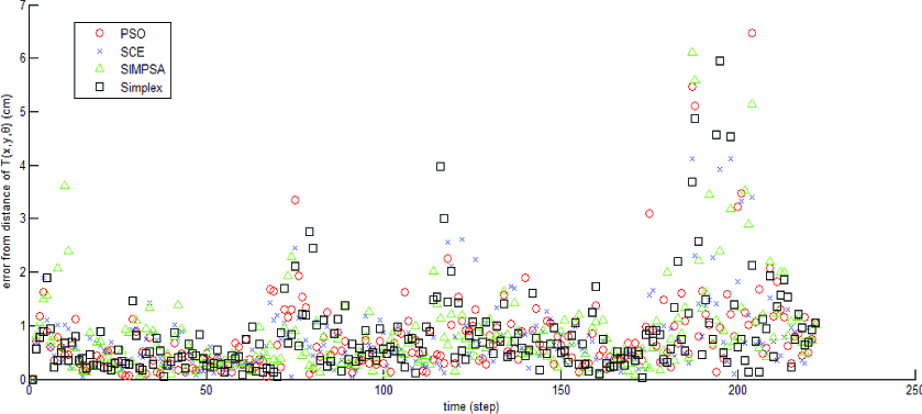
Errors of distance in transformation matrix.

Figure 9.

The distance from robot's position to the ground truth position

Table 1.

Errors of transformation matrix T(x,y,θ). û and ó show the average and standard deviation, respectively, of the error between the solutions obtained by each optimization method and global solution.

		Distance (cm)	X(cm)	Y(cm)	è°
PSO	Max	6.4657	2.5634	2.5634	0.5255
PSO	û±σ	0.77±0.81	0.34±0.35	0.61±0.79	0.094±0.09
SCE	Max	4.1131	1.9647	1.9647	0.6913
SCE	û±σ	0.74±0.67	0.35±0.31	0.57±0.67	0.099±0.09
SIMPSA	Max	6.1106	1.5526	1.5526	0.4835
SIMPSA	û±σ	0.83±0.83	0.36±0.31	0.65±0.85	0.10±0.088
Simplex	Max	5.9534	1.805	1.8052	0.7874
Simplex	û±σ	0.80±0.82	0.36±0.31	0.63±0.83	0.102±0.09

Table 2.

Errors of robot's position

		Distance to Ground-truth position (cm)	Relative Computational time (Methods/Simplex)
PSO	max	6.8941	99.7164
PSO	û±ó	2.8142±1.6403	99.7164
SCE	max	7.7390	8.0873
SCE	û±ó	3.5518±1.690	8.0873
SIMPSA	max	11.6108	4.1993
SIMPSA	û±ó	4.1986±3.0994	4.1993
Simplex	max	9.0126	1
Simplex	û±ó	3.6582±2.6818	1

3. 3D mapping system

The LRF scan takes only 2D measurements. The LRF needs a rotational motion to expand the 2D map to a 3D map. In this section we present a design of a rotational mechanism using a four-bar linkage to actuate the LRF for this purpose. During the 3D SLAM, we use the same horizontal information for each scan. The horizontal information can be detected from the first and last scans. The flow chart for the extension of 2D mapping to 3D mapping is shown in Figure 10. To transform the 2D data of a LRF to 3D data in each scan, the transformation is composed by interpolating TG and TL. The first step is to obtain an accurate linkage transformation TL(θ) of the rotation angle θ of the LRF. We compute the transformation matrix TG in our mapping system (Figure 5 and Figure 10), which transforms the map of the last scan to the map of the first scan, which is set as the global map. The details of the 3D mapping system and its testing are presented in this section.

Figure 10.

The flow chart of 3D mapping system

3.1 Mechanical design of rotational motion mechanism

Different rotational mechanism designs for 3D mapping robots have been presented with good functionality in practice [19 –21, 29 –31], For example, The mechanical design of a rotational motion of the LRF in [31] is an arm-type linkage., Our design of a crank-and-rocker four-bar linkage to actuate an LRF is presented in this subsection and its calibration is given in the Appendix. Figure 11(a) shows a four-bar linkage called a crank-rocker [32]. The sum of the shortest (s) and longest (l) links of the planar four-bar linkage must be smaller than the sum of the remaining two links (p, q). In this case the shortest link can rotate 360 degrees, relative to the longest link. As Figure 11(a) shows, a characteristic of the mechanism is that one link can rotate a whole circle continuously, while the rocker can undergo the motion of reciprocation (to and fro). Figure 11(b) shows a photo of our crank-rocker design, where the rocker should move slowly when the load is heavy, then return to moving quickly, as shown in: http://www.youtube.com/watch?v=RwwaWoePkUA&feature=related

Figure 11.

(a) The crank-rocker four-bar linkage (b) The rotational motion device. θ_input is the angle between linkages L₃ and L₂_. θ_output t (or θ* as its calibrated value) denotes the angle of the fixed linkage L7 relative to horizontal plane.

3.1.1 Linkage transformation

In the photo of our construction of the crank-rocker mechanism shown in Figure 11(b), the linkages (s, q, p, l) = (L3, L12, L5, L4) constitute a four-bar linkage and the other linkages L35, L6, L7 are fixed. The appendix shows the calibration of the linkages to ensure the accuracy of the movable sensor position and therefore the accuracy of the 3D mapping data acquired by this actuated LRF. The motor encoder is transformed to the rotational angle 0input of linkages L₃ and L₂ Then L35 and the angle θ_output between the fixed linkage L7 relative to the horizontal plane are derived using triangle theorem. By transforming the motor encoder to the angle θ* (i.e. the calibrated θ_output, defined in the Appendix) of the fixed linkage L7 relative to horizontal plane, the 2D range data (PLX, PLY) is obtained from rotating a LRF at different heights with the stationary robot. It is transformed to 3D data (PGX =PLX, PGY, PGZ) via (12):

$[\begin{matrix} P_{G X} \\ P_{G Y} \\ P_{G Z} \end{matrix}] = [\begin{matrix} 1 & 0 \\ 0 & \cos (θ^{*}) \\ 0 & \sin (θ^{*}) \end{matrix} \begin{matrix} 0 \\ 0 \\ 0 \end{matrix}] [\begin{matrix} P_{L X} \\ P_{L Y} \\ 1 \end{matrix}]$ (12)

Here we assume that the pose of stationary robot is (0,0,0).

3.1.2 Composite transformation

(12) derives the 3D data acquisition formula using a rotating LRF when the mobile robot is stationary. In a dynamic case, the robot travels along a path to a new scan location to take a new scan, so that a sequence of scans that contain new information in the map are constantly acquired and a local map is built for each scan to update the global map. The transformation matrix for a robot in motion is composed by two parts. First is the transformation matrix of the four-bar linkage that actuates the LRF. The other is the transformation matrix of a robot's localization. The transformation matrix of the four-bar linkage is the same for each scan, even when the robot is moving. For estimating the transformation matrix of robot localization, one needs the contrastive position of a sequence of acquired scans from the first scan (at t= t) to the last scan (at t=t+n). Given that the transformation matrix T_G = T_t^t⁺ⁿ (x_n,y_n,θ_n) in Figure 10 is defined by the first and the last scans, the transformation from the first scan to each intermediate scan when the robot is in slow motion is found by interpolation via:

$T_{t}^{t + i} (x_{i}, y_{i}, θ_{i}) = T_{G} \frac{i}{n}, i = 1, ..., n$ (13)

Combining the linkage transformation of the crank-rocker mechanism and the transformation of the moving robot pose (13), we obtain:

$\begin{array}{l} [\begin{matrix} P_{G X}^{t + i} \\ P_{G Y}^{t + i} \\ P_{G Z}^{t + i} \end{matrix}] = [\begin{matrix} \cos (θ_{i}) & - \sin (θ_{i}) & x_{i} \\ \sin (θ_{i}) & \cos (θ_{i}) & y_{i} \\ 0 & 0 & 1 \end{matrix}] \\ [\begin{matrix} 1 & 0 \\ 0 & \cos (θ^{*}) \\ 0 & \sin (θ^{*}) \end{matrix} \begin{matrix} 0 \\ 0 \\ 0 \end{matrix}] [\begin{matrix} P_{L X}^{t + 1} \\ P_{L Y}^{t + 1} \\ 1 \end{matrix}] \end{array}$ (14)

where the superscript denotes the time of the data and θ*is the linkage angle of the fixed linkage L₇ relative to horizontal plane defined in the Appendix. In this way, 2D data from the LRF is transformed to the global position in a 3D map via (14).

It is noted that (12) is a special case of (14).

3.1.3 System testing: stationary robot

For indoor navigation, the robot needs to recognize the objects in the environment. For testing the capability of our system for 3D object recognition when the robot stands still, three boxes are placed on the ground (see Figure 12(a)) and we construct their 3D maps, as shown in Figure 12(b). Since the length of each side of the boxes is an invariant, we compare the width (57.5, 34.8, 24.8 cm) with real measurement of boxes (58.29, 34.35, 25.2 cm) shown in Figure12(c). The discrepancies are 7.9, 4.5 and 4 mm in each dimension, due to the errors inherent in LRF sensing and the linkage transformation of the four-bar linkage.

Figure 12.

Stationary results of sensing 3D objects. (a) The scene of three boxes(b) The 3D map (c) 2D map by projecting 3D map of (b) onto X-Y plane (ground floor).

In another test, Figure 13 (a) and (b) show the same environment scanned at different locations using a stationary robot. There is an elevator far from the LRF and it is blocked by the walls in the central region of Figure 13(b). A plant contour of Figure 13(d) is constructed clearly in Figure 13(c). The edges of the windows can be seen clearly, but some of them are blocked. This experiment shows the limitation of 3D mapping using a rotating LRF mounted on a stationary robot, where the gathering of environment information is incomplete. To remedy this, the 3D information of the environment may be gathered more completely by a mobile robot equipped with a rotating LRF and by combining the moving robot pose and a linkage transformation.

Figure 13.

Stationary results. Two 3D mapping results produced by our mapping system fixed at different locations. Left:3D maps, Right: the scenes.

3.2 System testing: 3D mapping experiments

Figure 14 and Figure 15 are the results of experiments performed in the office buildings 3F and 7F, respectively. We eliminate all the information of the floor and ceiling to make the map visually clear. The running time of whole experiment is around 16 minutes. Figure 14(a) and Figure 15(a) are the results of GDT SLAM. Figure 14(b) and Figure 15(b) are the 3D maps which have been built. These maps are composed of the walls, together with some furniture in the middle space. The contour of the 3D maps is almost the same as the 2D maps. The film http://www.youtube.com/watch?v=ceBAgnJhack shows the details of the 3D map.

Figure 14.

Mapping result of 3F of IIS building.(a) GDT SLAM (b) The obtained 3D map.

Figure 15.

Mapping result of 7F of IIS building. (a) GDT SLAM (b)The obtained 3D map

Even though we demonstrate the accuracy and efficiency of the method for small movements of the mobile robot, the convergence of GDT SLAM is not attained in every situation. The convergence problem and comparison of our approach to other 3D mapping methods such as 6D SLAM [29, 21] are left for future work.

4. Conclusions

In this paper, we described the implementation and testing of a 3D robotic mapping system based on a scan matching method called simplex-based GDT SLAM. The local map is a grid map represented by a distance-transformation (DT) matrix. The range measurements during the 3D map building process could be facilitated by a rotational mechanism design of a crank-rocker four-bar linkage mounted on a mobile robot. The integrated system allows 3D scans of a rotating LRF to provide the height information, using a composition of linkage transformation and robot localization derived from a motor encoder and kinetic formula of the mobile platform and also allows the prediction of the 3D map. In the experiments performed in the office building for testing the 3D mapping system, the consistency, efficiency and accuracy of the mapping system are demonstrated by constructing 2D or 3D maps with a stationary or moving robot. For future work on real-time 3D mapping and the application scenarios based on it, the practical aspects of the compression and registration of huge 3D data using techniques such as 3D Normal Distributions Transform (NDT) of spatial representation of 3D point clouds [33] should be studied.

5. Appendix. The calibration of rotational motion

The measurement of the length of each linkage depicted in Figure 11(b) is shown below.

$\begin{array}{l} L_{1} = 13.2 + δ_{1}, L_{2} = 3.6 + δ_{2}, L_{3} = 12.5 + δ_{3}, L_{4} = 8.5 + δ_{4} \\ L_{5} = 8.8 + δ_{5}, L_{6} = 5 + δ_{6}, L_{7} = 11.8 + δ_{7} \end{array}$

In this Appendix, we describe the calibration of δ_i,i = 1,-,7in the tolerance interval [−0.5,0.5]cm for making the linkage transformation and thus 3D mapping acquisition, more correct. We set the mobile platform in front of a wall, which is supposed to be perpendicular to the floor. The rotating LRF performs a total of 500 scans, one scan for each 1.8° of rotation starting from θ=0° to 90° forward. We repeat this 200 times to collect 100,000 data points of range R_m(E_M)/angle θ(E_M) from two cycles of the motor encoder with 20,000 EM readings per cycle. The range data R_m(E_M) is plotted in Figure A(a) where R_m (0) is the distance value to the wall when the encoder reading is 0. We define the calibrated distance:

$R_{c} (E_{M}) = R_{m} (0) \cos (θ (E_{M}))$ (A1)

as shown in Figure A(b). The aim of calibration is to find δ_i,i = 1,…,7 such that:

$\arg \min_{δ_{i}} a b s (R_{c} (E_{M}) - R_{m} (E_{M}))$ (A2)

to yield a best fit calibration curve R*_c(E_M) (A1) with optimal θ*(EM) and R*_c(EM). Finally, the calibrated δ,i = 1,…,7 is obtained from minimizing (A2) as:

$\begin{array}{l} δ_{1} = 0.4034, δ_{2} = - 0.1178, δ_{3} = - 0.3218, δ_{4} = 0.2625 \\ δ_{5} = - 0.09, δ_{6} = 0.07, δ_{7} = - 0.1709 \end{array}$

Figure A.

Range data and motor encoder. (a) measured R_m(E_M) versus E_M (b) calibrated R_c(E_M) versus E_M

We use θ*(EM) as the rotational angle θoutput of a rotating LRF in Figure 11(b) for acquiring 3D mapping data in the experiments performed in this paper.

Footnotes

6. Acknowledgements

This work was supported by the National Science Council of ROC under contract NSC 99-2221-E-001-019.

References

Durrant-Whyte

and Bailey

(2006) Simultaneous localization and mapping: Part I. IEEE Robotics and Automation Magzine 13(2): 99–110.

Dissanayake

Newman

Clark

Durrant-Whyte

H.F

and Csorba

(2001) A solution to the simultaneous localization and map building (SLAM) problem. IEEE Trans. Robotics and Automation 17(3): 229–241.

Ouellette

and Hirasawa

(2007) A Comparison of SLAM implementations for indoor mobile robots. IEEE/RSJ International Conference on Intelligent Robots and Systems: 1479–1484.

Martinelli

Nguyen

Tomatis

and Siegwart

(2007) A relative map approach to SLAM based on shift and rotation invariants. Robotics and Autonomous Systems, 55(1): 50–61.

Mlford

M. J.

(2008) Robotic mapping methods. Robot Navigation from Nature, STAR 41: 15–28.

Werner

Maire

Sitte

Choset

Tully

and Kantor

(2009) Topological SLAM using neighborhood information of places. IEEE/RSJ International Conference on Intelligent Robots and Systems: 4937–4942.

Skrzypczynski

(2009) Simultaneous localization and mapping: A feature-based probabilistic approach. International Journal of Applied Mathematics and Computer Science: 19(4): 575–588.

Gutmann

J. S.

(2000) Robust navigation autonomer mobiler systeme. (in German) PhD thesis, Albert-Ludwigs University at Freiburg.

Hahnel

Burgard

Fox

and Thrun

(2003) An efficient FastSLAM algorithm for generating maps of large-scale cyclic environments from raw laser range measurements. IEEE/RSJ International Conference on Intelligent Robots and Systems: 206–211.

10.

Doucet

de Freitas

J. F. G.

Murphy

and Russell

(2000) Rao-Blackwellised particle filtering for dynamic Bayesian networks. Conference on Uncertainty in Artificial Intelligence

11.

Rofer

(2002) Using histogram correlation to create consistent laser scan maps. IEEE/RSJ International Conference on Intelligent Robots and Systems.

12.

Skrzypczynski

(2009) Simultaneous localization and mapping: A feature-based probabilistic approach. AMCS 19 (4): 575–588.

13.

Besl

P. J.

and McKay

N. D.

(1992) A method for registration of 3D shapes. IEEE Transactions on Pattern Analysis and Machine Intelligence 14(2): 239.256.

14.

and Milios

(1997) Globally consistent range scan alignment for environment mapping. Autonomous Robots: 333–349.

15.

Mihankhah

Taghirad

H.D.

Kalantari

Aboosaeedan

and Semsarilar

(2009) Line matching localization and map building with least square. IEEE/ASME International Conference on Advanced Intelligent Mechatronics: 1734–1739.

16.

Yaqub

Tordon

M.J.

and Katupitiya

(2006) Line segment based scan matching for concurrent mapping and localization of a mobile robot. 9^th International Conference on Control, Automation, Robotics and Vision: 1–6.

17.

Murty

K. G.

(1983) Linear programming. John Wiley & Sons. New York.

18.

Wulf

and Wagner

B. A.

(2003) Fast 3D scanning methods for laser measurement systems. International Conference on Control Systems and Computer Science 1: 312–317.

19.

Xiang

and Wu

(2006) Design and calibration of a fast 3D scanning. LADAR, International Conference on Mechatronics and Automation: 211–215.

20.

Zhang

and Chen

(2008) Fast continuous 360 degree color 3D laser scanner. The International Archives of the Photogrammetry, Remote Sensing and Spatial Information Science XXXVII (Part B1): 409–414.

21.

Bosse

and Zlot

(2009) Continuous 3D scan-matching with a spinning 2D laser. IEEE International Conference on Robotics and Automation: 4312–4319.

22.

Elseberg

Borrmann

and Nüchter

(2012) 6DOF semi-rigid slam for mobile scanning. IEEE/RSJ International Conference on Intelligent Robots and Systems

23.

de la Puente

Valero

and Rodriguez-Losada

(2009) 3D mapping: testing algorithms and discovering new ideas with USARSim. Robots, Games, and Research: Success stories in USARSim. IEEE/RSJ International Conference on Intelligent Robots and Systems

24.

Kennedy

and Eberhart

(1995) Particle swarm optimization. IEEE Int. Conf. on Neural Networks: 1942–1948.

25.

Cardoso

M. F.

Salcedo

R. L.

and De Azevecoo

S. Fevo

(1996) The simplex-simulate annealing approach to continuous non-linear optimization. Computers Chem. Eng 20(9): 1065–1080.

26.

Duan

Q. Y.

Gupta

V. K.

and Sorooshian

(1993) Shuffled complex evolution approach for effective and efficient global minimization. Journal of Optimization Theory and Applications 76(3): 501–521.

27.

Breu

Gil

Kirkpatrick

and Werman

(1995) Linear-time Euclidean distance transform algorithms. IEEE Transactions on Pattern Analysis and Machine Intelligence 17(5): 529–533.

28.

Thrun

Burgard

and Fox

(2000) A real-time algorithm for mobile robot mapping with applications to multi-robot and 3D mapping. IEEE International Conference on Robotics and Automation.

29.

Surmann

Lingemann

Nuchter

and Hertzberg

(2001) A 3D laser range finder for autonomous mobile robots, 32^nd International Symposium on Robotics: 153–158.

30.

Michalicek

Klimentjew

and Zhang

(2011) A 3D simultaneous localization and mapping exploration system. 2011 IEEE International Conference on Robotics and Biomimetics: 1059–1065.

31.

Fujita

(2012) 3D sensing and mapping for a tracked mobile robot with a movable laser range finder. International Journal of Electronics and Electrical Engineering 6: 243–268.

32.

Molian

(1982) Mechanism design: an introductory text, Cambridge University Press.

33.

Stoyanov

Magnusson

Andreasson

and Lilienthal

A.J.

(2012) Fast and accurate scan registration through minimization of the distance between compact 3D NDT representations. International Journal of Robotics Research: online first.

34.

Hou

J.-F.

Chou

Y.-S.

Chang

Y.-Z.

Liu

J.-S.

(2010) Experimental investigation of a prediction algorithm for an indoor SLAM platform. 2010 International Conference on Intelligent Robotics and Applications (2): 154–165