Sage Journals: Discover world-class research

Abstract

Energy efficiency is very important for wireless sensor networks (WSNs) since sensor nodes have a limited energy supply from a battery. So far, a lot research has focused on this issue, while less emphasis has been placed on the adaptive sleep time for each node with a consideration for the application constraints. In this paper, we propose a hierarchically coordinated power management (HCPM) approach, which both addresses the energy conservation problem and reduces the packet forwarding delay for target tracking WSNs based on a virtual-grid-based network structure. We extend the network lifetime by adopting an adaptive sleep scheduling scheme that combines the local power management (PM) and the adaptive coordinate PM strategies to schedule the activities of the sensor nodes at the surveillance stage. Furthermore, we propose a hierarchical structure for the tracking stage. Experimental results show that the proposed approach has a greater capability of extending the network lifetime while maintaining a short transmission delay when compared with the protocol which does not consider the application constraints in target tracking sensor networks.

Keywords

Energy Efficiency Target Tracking WSN

1. Introduction

In a wireless sensor network (WSN), sensor nodes are always deployed in an unattended natural environment and are of an enormous amount. It is unfeasible to replenish their energy by replacing their battery after deployment. Therefore, reducing energy consumption to prolong the life of the network is the most critical issue in WSN.

Power management (PM) is an efficient way to conserve energy after the sensor nodes have been deployed [1]. The main idea of PM is to dynamically make the nodes sleep to reduce their energy consumption. The PM has to decide when a sensor node should go to sleep and the amount of time to stay so. In order to devise a more efficient PM mechanism, the application constraints should be considered, mainly in sensor networks that strongly depend on an application. In target tracking sensor network, the users are only interested in the occurrence of a certain event. These interesting events do not happen frequently and they commonly have long intervals of inactivity. Specifically, the target tracking scenario can be divided into two stages, namely, surveillance and tracking. During the surveillance state, there is no target of interest in the sensing field, but the sensors are ready to detect any possible occurrences. While in the tracking stage, the network reacts in response to any moving targets, and collectively track and record the roaming path of a moving target. As such, when no target appears, it would be a significant waste of energy if all the nodes always remained active. Moreover, a target moves randomly in the sensing field. We do not know the next position of the target. If we blindly turn the sensor node off during each idle period, we will miss some events or waste more energy.

A lot of pioneering research in the area of energy conservation for WSNs has focused on dynamic power management (DPM) schemes to minimize the energy consumption of sensor nodes, such as [3, 4, 5]. However, the existing works have the follow limitations: (1) the sleep period of sensor nodes cannot change based on the position of the target. As a result, many nodes far away from the target consume energy in active mode, but they do not detect a target. (2) In the coordinate PM approach, when a node decides if it should go into sleep state, it will use the detected information from its neighbours in order to exactly estimate if the target will be in its sensing area in the next instant. Due to dense nodes in WSNs, the information from adjacent nodes is similar and related. If every node sends the detected information to its neighbours, lots of energy will be wasted and, at the same time, it will result in information redundancy. (3) It is difficult to have both energy conservation and transmission delay reduction. Since the sensed data is sent to the sink by multi-hop routing, more nodes are in the sleep state and longer delays are introduced in the packet delivery because during the sleep phases nodes cannot communicate and packets cannot be transmitted until the relay or destination nodes wake up.

With these issues in mind, we propose a hierarchically coordinated power management (HCPM) approach that considers the application constraints in order to exploit sleep and active intervals. Our main goal is to choose an optimal sleep time for each node so as to make the system adaptive and energy-efficient. We manage the power of sensor nodes based on a grid-based network structure, which divides the entire sensing field into virtual grids. In each grid, one node is selected as the grid head (GH) and others are grid members (GMs). It is a simple, scalable and efficient method for the implementation of WSN applications [1, 2, 16 –19]. In recent works, grid-based sensor network architecture has been widely used, such as for data gathering [16, 17], network coverage [1, 2], and other applications [18]. In my work, dividing the network into grid based on the geographical information is a highly efficient method because the tracking application always relates to the geographical position of the target. In detail, the contributions of this paper are three aspects:

Proposing a new adaptive PM approach: our approach combines the fixed sleep and adaptive sleep interval. In each grid, one node is selected as the grid head (GH) and others are grid members (GMs). The GH adopts the local PM policy and the fixed sleep interval to maintain synchronization and reduce the data transmission delay, whereas the GMs adopt an adaptive sleep time according to their position to save energy.

Better balancing of the energy consumption of sensor nodes: when there is no target, the interior nodes can sleep more because the GMs have an adaptive sleep time according to the distance between the grids and the network border so that the energy consumption between the fringe and interior nodes are balanced since the interior nodes always take on more relay tasks.

Proposing a hierarchical structure: in the tracking stage, the network can be divided into several sub-areas. Only one sub-area uses the tracking stage sleep policy, while others can still use the surveillance sleep policy. This makes the network more adaptive and energy efficient.

The rest of this paper is organized as follows: Section 2 gives an overview of related works. Then, Section 3 states the specific problem. After that, the proposed approach is described in detail in Section 4. The experimental results are shown in Section 5. Finally, we conclude the paper in Section 6.

2. Related Works

To achieve a satisfactory network lifetime, several methodologies have been proposed at the hardware and system levels [3][4] to design energy efficient communication processes. In addition, DPM schemes have been proposed to reduce power consumption [5][6].

The simplest method of PM for sensor nodes is using a Fully Synchronized Pattern [7]. In this case all nodes wake up periodically every wake-up instant for a fixed time. Then, they return to sleep until the next wake-up instant. In [8], a further improvement was achieved with the local PM approach, which allows nodes to switch off their radio when no activity is detected for at least a timeout value. Each node keeps a timer to record how long no event has been detected and goes to sleep after this timer times out. However, these schemes are not very flexible since the size of the sleep and active periods is fixed and does not adapt to variations in the target tracking application scenario.

The ideal PM for target tracking is the on-demand scheme, in which a node should be woken only when it needs to execute its task. The implementation of such schemes typically requires two different channels: a data channel for normal data communication and a wakeup channel for awaking nodes when needed, such as in [9]. Unfortunately, this scheme is almost always impractical because it can be only applied when the distance between nodes is very short (a few metres). Moreover, the wakeup radio is costly and generally it is not provided with commonly used sensor platforms.

The authors in [10] propose an adaptive coordinate PM policy, which extends the local PM decision to include the timeout values of the neighbours in the network. In this way, nodes will be aware of the timeout status of their neighbours, and can enter into low-power mode if it and each of its neighbours are simultaneously in a timeout state. In [11], a voting PM policy is proposed. Each node broadcasts detected information periodically and collects this information from its neighbours. If enough of the neighbours vote there is no target being detected, then the node enters the sleep state. However, due to the dense nodes in WSNs, the nodes in an adjacent area have similar detected information. If every node broadcasts its detected information to its neighbours, it results in more transmission energy consumption and information redundancy.

In [12], the authors dynamically change the sleep schedule of sensor nodes by considering how many hops there are from the node to the target. However, when a node far from the sink detects a target, it has to wait until the nodes which are far from the target and close to the sink to wake up before it can transmit its data. Thus, there will be a long data transmission delay. In [13], the authors propose the Staggered Sleep Pattern which divides time into cycles based on a time synchronization method. However, for target tracking, this method is not energy efficient because all the sensor nodes have to be woken up each cycle; nevertheless, not all of the nodes will sense the target and the implementation of global synchronization is not easy and consumes lots of energy. In [14], asynchronous schemes allow each node to wake up independently by guaranteeing that the active periods of their neighbours will always have overlapped within the specified cycles. Although, this protocol does not need a tight synchronization, it usually results in a higher duty cycle for sensor nodes than synchronous counterparts.

Furthermore, to switch off the idle nodes, some prediction algorithms were developed to predict the target movement in [15]. Nevertheless, the prediction algorithms are always implemented at the sink in a centralized way with high computation complexity and communication energy cost. This results in a lot of communication between sensor nodes and the sink which consumes lots of energy.

3. Problem statement

In the target tracking application, if a target appears within the sensing area of a node, the node should be awake in advance in order to sense the target and transmit data, if not, the tracking performance is reduced. However, the power consumption in sleep state is usually much lower than in the active or idle mode. Thus, the sensor nodes may be put into a sleep mode as long as possible in order to conserve energy. In this paper, it is assumed that a sleep node cannot be communicated with or woken up so a decision to put a node to sleep implies that this node cannot be scheduled at a future time until it wakes. So estimating when sensor nodes should go to sleep and the idle time of nodes are crucial in PM.

On one hand, if all the sensor nodes adopt the same and fixed sleep policy, lots of nodes will be in the idle state and they will consume a lot of energy and will not detect any targets. Therefore, this method is not suitable for a target tracking application scenario where a target moves dynamically, which only needs a portion of the nodes near to the target to work whilst the other nodes can be in sleep state. Therefore, each node should be assigned the maximum sleep time to save energy. Theoretically, to guarantee the tracking performance, the maximum sleep time of the node N_i is calculated by the following equation,

t_{\max} = \frac{\sqrt{{(x_{targ} - x_{i})}^{2} + {(y_{targ} - y_{i})}^{2}} - R_{s e n s e}}{v_{\max}} - τ_{d} - τ_{u}

(1)

where (x_targ, y_targ) is the location of the target, and (x_n, y_n) is the location of node N_i. R_sense is the sensing range of the sensor node. v_max stands for the possible maximum velocity of the target and it is decided by an application scenario. τ_d is the transition time from idle state to the sleep state and τ_u is the transition time back.

On the other hand, if all the sensor nodes adopt a sleep time appropriate to the position of the target, each node has a different sleep interval and an asynchronous wakeup instant. It results in a longer data transmission delay that is also a critical issue to be considered in the nodes' sleeping policies. The delay is defined as the time between the moment a source sends a packet and the moment a sink receives the packet. When a node wants to send data, it has to wait until the relay nodes wake up from the sleep mode so that there will be a long delay for data transmission in a multi-hop manner. In detail, the delay can be calculated as,

d_{t r a n s} = \sum_{h = 1}^{H} (t_{l, h} + S_{l, h} τ_{u} + t_{p r o c, h} + t_{t r a n s, h})

(2)

Where H is the number of hops from the data source node to the sink, and t_l,h is the remaining sleep time of the h-th hop node at time l. S_l,h denotes the state of the hth hop node at time l, if the node is active or idle, S_l,h = 0, otherwise, S_l,h = 1. t_proc,h and t_trans,h are respectively the process and the transmission time at the h-th hop node. From Equation (2), we can see that the longer the sleep time of the node, the longer the data transmission delay that occurs. Moreover, if the sensor nodes have synchronized active time, there is a relatively small transmission delay.

So we see that the task is to find the most efficient method with which to assign the sleep time to the sensor nodes under the given application constraints so that the total network lifetime is extended with less data transmission delay.

4. Hierarchically Coordinated PM Approach

A. Network Model

We consider a static WSN which is composed of one sink and some randomly and evenly distributed sensor nodes N_i, i ∈ [1, n] in a two-dimensional sensing field, where n is the number of the deployed nodes. The sink is assumed to have an infinite power supply and it gathers sensed information from sensor nodes. The nodes distribution is mutually independent with density λ = n/S_sens, where S_sens is the area of the sensing field. We assume each node is aware of its location after deployment (e.g., using some localization techniques) [21]. Let X_i(x_i, y_i), 1 ≤ i ≤ n be the location of node N_i.

Figure 1.

Illustration of a grid structured sensor network

Furthermore, the whole sensing field is divided into small equally sized grids and in each grid one node with the most energy is selected as the GH. The network is organized as shown in Fig. 1. In the definition of this virtual grid, each pair of nodes in the neighbouring and diagonal grids can directly communicate with each other [1, 2]. Let us assume the transmission range of a sensor node is R_t. The size of each grid is α × α. In any two adjacent grids, the distance between the two possible farthest nodes must not be larger than R_t. Therefore, we get:

{(2 α)}^{2} + {(2 α)}^{2} \leq R_{t}^{2} or α \leq \frac{R_{t}}{2 \sqrt{2}}

(3)

Initially, all the sensor nodes are in the idle state and they have the same initial energy. One node in each grid is randomly selected as the GH by broadcasting an announcement (carrying its position and grid ID) after waiting for a random time period R(T_ran), which is a discrete random variable with the uniform distribution in [0,T_ran]. The first node to broadcast its GH announcement in a grid will be the GH. After the process, there is one GH in each grid. In addition, each grid has a grid ID, and the nodes in one grid have the same grid ID. A sensor node can calculate its grid ID (u, v) from its location X_i(x_i, y_i) as:

u = [\frac{x_{i} - x_{0}}{α}], v = [\frac{y_{i} - y_{0}}{α}]

(4)

where [] is a symbol which stands for the integer part of the number in it. (x₀, y₀) is the location of the network origin, which is a system parameter set in the network initialization stage. For the sake of simplicity, we assume that u and v are positive. From the initial process, each node can learn information about other nodes in the same grid and keep the information, e.g., the location and so on.

B. Sleep State Transition Model

In this paper, the sensor nodes have three states, active, idle and sleep state. In the active state, the nodes sense the target, and send and receive data. In the idle state, the node prepares for detection and receives messages from others. While in sleep mode, the sensor node cannot execute any function and it cannot be woken up externally but instead has to set an internal timer to determine the next time to wake.

Figure 2.

Sleep states transition latency and power

Fig. 2 shows the power-time curves for the transition of the sleep states. Each sleep state S_k has power consumption P_k. The transition time from the active state and back are denoted by τ_d and τ_u, respectively. From that we can see that the sleep state has less power consumption but incurs latency and needs energy to awaken. Let us assume an event is detected by node N_i at a given moment in time. N_i finishes processing the event at time t₁ and predicts the next event will occur at time t₂= t₁ + t_i+ τ_u. At time t₁, N_n decides to transfer to sleep. So a sleep time threshold T_th,k can be utilized to avoid losing the event,

T h_{1} = τ_{d} + τ_{u}

(5)

If (t₂- t₁)> Th₁, N_i can go to sleep state S_k at time t₁ and wake up at t₂. Otherwise, when (t₂- t₁) ≤ Th₁, N_i should not. So the energy saved from a state transition can be calculated as follows,

E_{s a v e, k} = P_{i} (t_{i} + τ_{d}) - \frac{P_{i} + P_{s}}{2} (τ_{d} + τ_{u}) - P_{s} (t_{i} - τ_{u})

(6)

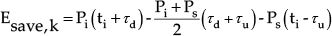
The energy saving makes sense when E_{save, k}> E_c, where E_c is the additional energy consumption for the sleep state transition. So we can work out the threshold,

T h_{2} = \frac{E_{c} + P_{t r^{1}} τ_{d} + P_{t r^{2}} τ_{u} - P_{i} (τ_{d} + τ_{u})}{P_{i} - P_{s}}

(7)

where P_i, P_s P_tr¹ and P_tr2 are the power consumption in the idle, sleep and transition state from active to sleep state and back, respectively.

C. Power Management in the Surveillance Stage

During surveillance time, though there is no target in the sensing area, all the sensor nodes should remain at a certain level of vigilance to get ready for detecting. When a target enters into the sensing area, it has to pass through the borders of the area. For this reason, to avoid missing the target and to have less energy consumption, it is only necessary for the sensor nodes in border grids to stay alert and for the nodes in interior grids to have more sleep time as shown in Fig. 3. Each GH stays active in order to transmit data and the GMs in each grid have the same sleep/awake period. The sleep time of GMs is adaptively adjusted by their GH according to the distance from the grid to the network border. The further the grid from the network border, the more sleep time the GMs have. Lj (j=1, 2…) is the layer of the grid.

Figure 3.

The PM in surveillance stage

At the initial stage, each GH calculates the sleep time for its GMs and informs them of this. In each period, the GH decides if the sleep time of its GMs needs to be changed based on the information received or detected (e.g. if the GH received the detected information from one of its GMs). If needed, the GH will send a new sleep time value to its GMs, otherwise, the GMs will keep the same value for their sleep period as before. When there is no target, the GMs stay in the sleep mode according to the sleep time value received from their GH and wake up at certain time slot to detect if a target has appeared and to receive a new sleep time value from their GH. To meet the requirements of the applications and not miss the target, the maximum sleep time t_bord of the GMs in border grid can be calculated as follows,

t_{b o r d} = \frac{R_{b o r d}}{v_{\max}}

(8)

where R_bord is the side length of the sensing area of the nodes at the border grids. According to (5) and (7), when t_bord ≥ _Th₁ and t_bord > _Th₂ holds, the sleep time of the GMs in the border grids can be set as t_bord, otherwise it is 0.

As the distance between grids and the network border increases, the GMs can be allocated more sleep time to save energy and GMs in the different grids can have different sleep time schedules. In the interior grids, the GHs calculate the maximum sleep time for the GMs in a grid in Lj as follows,

t_{inter} = \frac{d_{\min}}{v_{\max}} = \frac{(j - 1) α}{v_{\max}}

(9)

where d_min is the shortest distance from the current grid to the border.

Similarly, when t_inter ≥ Th₁ and t_inter > Th₂ holds, the sleep time of the GMs in the interior grids can be set as t_inter, otherwise it is 0.

When one fringe node detects a target, it can report the information of the moving target to its GH with less delay. Then, the GH can inform its neighbouring GHs to re-arrange the sleep time for their GMs. This method not only conserves more energy but also grantees target detection. Moreover, it can balance the energy consumption between the border and the interior nodes since the nodes in interior grids always take more relay tasks. This scheme does not require global synchronization and synchronization within a grid is not difficult with the coordination of the GH. At the same time, the sensed data can be reported to the sink through multiple GHs with less transmission delay.

D. Power Management in the Tracking Stage

In the tracking stage, the GHs have the same PM policy as that in the surveillance stage. When a target appears, the node which detects the target first reports the detected information “target_detected” to its GH. Also, the GMs in the same grid as it overhear this message instructing them to stay active for detecting. When the detected information reaches the GH which will stay active in the next periods, it will be sent to the sink by the other GHs. The sink will inform all the GHs to change to the tracking stage. Since the detected information is forwarded only by the GHs instead of involving all the nodes, this can save significantly on energy. Later, all the nodes will go into the tracking stage. When the target moves out of the sensing field, the sink will send the message “no_target” to all the GHs. Then, all the nodes will go back to the surveillance stage. The transition between the surveillance and the tracking stage is shown in Fig. 4.

Figure 4.

Transition between the surveillance and the tracking stage

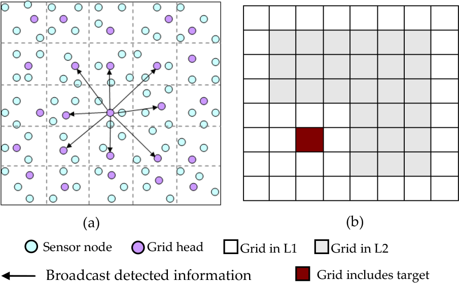
For the surveillance stage, the sleep time of the GMs is decided by the distance from the grid to the network border, whereas for the tracking stage, the sleep time of the GMs is decided by the both the distance between the grid and the network border and the distance between the grid and the target. Since the position of the target is not known by all the nodes, every CM should stay alert and have a short sleep time t_bord which should be the same as that of the border GMs, to detect the target. In a centralized manner, the sink informs each node of the target's location information so that the node can choose a proper sleep time according to the information received from the sink. However, it results in a high communication energy cost when the target moves. In our approach, the local information is used instead of the global information. Because the target is continuously moving, the sleep time of each node must be adjusted accordingly. When the target is in the node's sensing range, in order to wake up in time, each node can use the results of the motion detection from its neighbours in a coordinated manner. Each node broadcasts its detected information to its neighbours periodically. When the current node decides if it should go to the sleep state, it will use the detected information from its neighbours. However, due to the dense nodes in WSNs, the nodes in an adjacent area have the similar detected information. If every node broadcasts its detected information periodically, it will result in more transmission energy consumption and information redundancy. In our approach, only the GH which detects a target or receives the target information from its GMs broadcasts the detected information to its neighbouring GHs. We divided the grids into three parts: 1) the tracking grid, which includes the target. The GMs in the grid is active for detecting; 2) the neighbouring coordinated grid, the GH of which can receive the detected information from the GH of the tracking grid; 3) the guarding grid, which is at the network border and always stays alert.

Detected information is broadcasted by the GH which detects a target or receives the detected information from its GMs. When a GH makes PM decisions, it just considers the detected information from its immediate neighbouring GHs (shown as Fig. 5). If a GH does not receive the detected information, it can ascertain that the distance from the target to itself is larger than the side length of one grid α. A GH calculates the sleep time for its GMs in three different cases. The work process of the GHs is shown in Algorithm 1.

The first case is that the GH neither detects any target nor receives any target information from the others during a given time period. The maximum sleep time of the GMs is decided by the following equation,

t_{t r a c} = \frac{α}{v_{\max}}

(10)

The second case is that the target is detected by the GH or its GMs. The GH remains active until the target moves out of the sensing area of its grid and it decides the sleep time of its GMs t_trac = 0. Then the GH broadcasts a detected information message to its neighbouring GHs so that they can prepare to track the target at the next moment.

The third case is that the GH receives the target information from its neighbours. Thus, the GH can calculate the maximum sleep time for its GMs with the following equation,

t_{t r a c} = \frac{R_{b o r d}}{v_{\max}}

(11)

Similarly, when t_trac ≥ Th₁ and t_trac > Th₂ holds, the sleep time of the GMs in the tracking stage can be set as minimum {t_trac, t_surv}, in which t_surv is the sleep time of the GMs in the surveillance stage, otherwise it is 0. Each GH can decide if the sleep time of its GMs needs to be changed based on the information it received. When there is a change to the sleep time value of GMs, the GH informs its GMs about the updated sleep time in the next active instant. The GMs receive a new sleep time from their GH and adjust their current sleep mode adaptively.

Figure 5.

The PM in tracking stage

In this way, sensor nodes will get the target movement information from the GHs in a neighbouring area and accurately estimate the sleep state and time interval. In addition, transmitting the target information only among the GHs instead of among all the sensor nodes can reduce the communication costs and information redundancy.

1. (a) The work process of GHs 2. if a target is detected then 3. inform its neighbouring GHs 4. inform its GMs 5. otherwise if it receives (“target information”) from its GMs then 6. inform its neighbouring GHs 7. otherwise if it receives (“target information”) from neighbouring GHs then 8. t_sleep ← CalculateSleepTime(“target information”) 9. Broadcast (“new_sleepTime”) 10. end if 11. 12. (b) The work process of GMs 13. setTimer(ACTIVE_TIMEOUT, t_active) 14. if a target is detected then 15. CancelTimer(ACTIVE_TIMEOUT) 16. otherwise if it receives (target information) from its GH or the GMs in the same grid then 17. CancelTimer(ACTIVE_TIMEOUT) 18. otherwise if it receives (“new_sleepTime”) from its GH then 19. t_sleep ← GetNewSleepTime(“new_sleepTime”) 20. end if 21. while active time expires do 22. ChangeRadioStateTo(SLEEP) 23. setTimer(SLEEP_TIMEOUT, t_sleep) 24. end while 25. while sleep time expires do 26. ChangeRadioStateTo(ACTIVE) 27. end while

Algorithm 1. The Coordinated PM in tracking stage

E. Hierarchical structure

If the whole sensing area is relatively big, when a target enters into the sensing area from one network border, if all the sensor nodes change to the tracking sleep policy, a lot of energy will be wasted, which is not necessary since the nodes are far from the target. For this case, we propose a hierarchical structure as Fig. 6 and Fig. 7 shows. When the sink receives the message that the target is detected for the first time, the sink informs all the GHs of the position of the target and the sub-areas information. The whole sensing area is divided into several sub-areas. Each GH calculates the sleep time for its GMs according to the sub-area it is in. The tracking sub-area uses the sleep policy of the tracking stage, whereas the surveillance sub-area still adopts the sleep policy of the surveillance stage. This means that the nodes which are far from the target can still maintain the surveillance state to save more energy.

Figure 6.

Hierarchical structure

Figure 7.

Hierarchical structure

We assume the size of the network is M × M. Thus, the number of grids on one side of the network border is,

K = \frac{M}{α}

(12)

For the simplicity of the analysis, we assume K=2ⁱ, (i=1, 2, 3…) so that the network can be divided effectively, as in Fig. 9. In the surveillance sub-area, the summation of the sleep time of all the GMs is,

t_{s u r v} = (8 L - 4) N_{C} t_{s l e e p}^{s_F G} + \sum_{l = 2}^{L} [(L - l + 1) \times 8 - 4] N_{C} t_{s l e e p^{l}}^{s_I G}

(13)

where N_C is the average number of the GMs in each grid, and L is the number of the grids from the sub-area border to the canter. t^s_FG_sleep and t^s_IG_sleep¹ are the sleep time of the sub-area border GMs and the l-layer interior GMs, respectively.

By combining Equations (8), (10) and (11), Equation (13) is rewritten as,

\begin{array}{l} t_{s u r v} = (8 L - 4) N_{C} \frac{R_{b o r d}}{v_{\max}} + \sum_{l = 2}^{L} [(L - l) 8 + 4] N_{C} \frac{(l - 1) α}{v_{\max}} \\ = N_{C} \frac{R_{b o r d}}{v_{\max}} (8 L - 4) + N_{C} \frac{α}{v_{\max}} (\frac{4}{3} L^{3} - 2 L^{2} + \frac{2}{3} L) \end{array}

(14)

Due to $L = \frac{K}{2^{g}} (g = 2, 3 \dots G)$ , where G is the grades by which the network is divided, therefore,

\begin{array}{l} t_{s u r v} = N_{C} \frac{R_{b o r d}}{v_{\max}} (8 \frac{K}{2^{g}} - 4) + \\ + N_{C} \frac{α}{v_{\max}} (\frac{4}{3} \frac{K^{3}}{2^{3 g}} - 2 \frac{K^{2}}{2^{2 g}} + \frac{2}{3} \frac{K}{2^{g}}) \end{array}

(15)

Moreover, in the tracking sub-area, the summation of the sleep time of all the GMs is,

\begin{array}{l} t_{t r a c} = (8 L - 4) N_{C} t_{s l e e p}^{s_F G} + N_{C} t_{s l e e p}^{t k} \sum_{l = 2}^{L} [(L - l) 8 + 4 - N_{t}] \\ = (8 L - 4) N_{C} \frac{R_{b o r d}}{v_{\max}} \\ + N_{C} \frac{α}{v_{\max}} (4 L^{2} - (8 + N_{t}) L + 4 + N_{t}) \end{array}

(16)

where N_t is the number of nodes which are active and tracking a target. In the tracking sub-area, L = K / 2^G

\begin{array}{l} t_{t r a c} = (8 \frac{K}{2^{G}} - 4) N_{C} \frac{R_{b o r d}}{v_{\max}} \\ + N_{C} \frac{α}{v_{\max}} [4 \frac{K^{2}}{2^{2 G}} - (8 + N_{t}) \frac{K}{2^{G}} + 4 + N_{t}] \end{array}

(17)

Therefore, the total sleep time of the network is,

\begin{array}{l} t_{s u m} = \sum_{g = 2}^{G} 3 t_{s u r v} + t_{t r a c} \\ = \frac{3 N_{C}}{v_{\max}} \sum_{g = 2}^{G} [R_{b o r d} (\frac{8 K}{2^{g}} - 4) + \frac{2}{3} α (\frac{2 K^{3}}{2^{3 g}} - \frac{3 K^{2}}{2^{2 g}} + \frac{K}{2^{g}})] \\ + N_{C} \frac{α}{v_{\max}} [\frac{4 K^{2}}{2^{2 G}} - (8 + N_{t}) \frac{K}{2^{G}} + 4 + N_{t}] \\ + (\frac{8 K}{2^{G}} - 4) N_{C} \frac{R_{b o r d}}{v_{\max}} \end{array}

(18)

After further calculation, we can obtain,

\begin{array}{l} t_{s u m} = \frac{N_{C} R_{b o r d}}{v_{\max}} (K (12 - \frac{16}{2^{G}}) + 8 - 12 G) \\ + \frac{N_{C} α}{v_{\max}} (N_{t} + 4) + \frac{N_{C} α}{v_{\max}} [\frac{1}{14} K^{3} (1 - \frac{1}{8^{G - 1}}) \\ + \frac{1}{2} K^{2} (\frac{3}{4^{G - 1}} - 1) + K (1 - \frac{10 + N_{t}}{2^{G}})] \end{array}

(19)

Therefore, the average energy saved by GMs sleeping is,

E_{s} = \frac{(P_{i} - P_{s}) t_{s u m}}{K^{2} N_{C}} - (P_{t r^{1}} - P_{s}) τ_{d} - (P_{t r^{2}} - P_{s}) τ_{u}

(20)

If the target moves out of a tracking sub-area, the sink will inform the GHs in the tracking sub-area to change into the surveillance state and inform the surveillance sub-area where the target moves into transit to the tracking state. In this way, the average energy consumption of the state transition of the tracking and surveillance sub-area is,

E_{t} = (\frac{t_{s u m}}{K^{2} N_{C}} / \frac{K α}{v_{\max} 2^{G}}) \frac{K^{2} (E_{b r} + 8 E_{r e} + N_{C} E_{r e})}{K^{2} N_{C}}

(21)

Combining Equations (33), (34) and (35), when the parameters and application scenario is determinate, we can obtain the net energy saving is,

E_{s} - E_{t} = f (K, G)

(22)

According to Equation (36), the relation of (E_s, E_t) and (K, G) can be drawn as in Fig. 8. We can choose G based on the optimal energy saving.

We also further prove our results in an intuitionistic manner. As Fig. 9 shows, when K=8, the energy consumption is optimal if the hierarchical grade G is 1, however, if G=2, the number of grids the members of which are in L1 is increased so that the total sleep time of the GMs is decreased.

Figure 8.

The relation of K and G

Figure 9.

Hierarchical structure when K=8

F. Grid Maintenance

To avoid that a GH overfull consumes energy, if the energy of any GH is lower than a threshold T_e, the GH will broadcast a message “req-replace” to its GMs. Then the nodes in the same grid reselect the GH. A node with more remaining energy is selected to become a new GH.

The pseudo code of the GH selection is shown in Algorithm 2. When a GM receives the “req-replace” message, it waits a random time to broadcast the “finish_election” message to compete the GH election. Each GM's residual energy Eⁱ_residual is converted to a waiting time T_i (line 4). More residual energy leads to a shorter T_i. Therefore, the GM with the most Eⁱ_residual waits for the shortest time before sending the “finish_election” message to others. Therefore, it can be selected as the GH. (Line 8 and 12). The other nodes stop waiting and give up the GH election as soon as they receive the message. T_i is calculated by the following equation:

T_{i} = T_{m i n} + (T_{m a x} - T_{m i n}) (1 - \frac{E_{r e s i d u a l}^{i}}{E_{i n i t i a l}^{i}}) + R (T_{r a n})

(23)

where T_min and T_max are two design parameters, which are used to control the waiting time in a reasonable range. Eⁱ_residual and Eⁱ_initial are the residual and initial energy, respectively, of the node. Eⁱ_residual is divided by Eⁱ_initial in order to avoid a situation of a node waiting for too much time when its residual energy becomes very low. Two nodes might have the same residual energy and communication costs and therefore have the same T_i. To avoid this a random time R(T_ran) is added. R(T_ran) is a discrete random variable with uniform distribution in [0, T_ran], which is an order of magnitude smaller than T_max. In this paper we set T_min, T_max and T_ran to be 10⁻⁴ seconds, 10⁻² seconds, and 10⁻⁵ seconds, respectively.

1. while(after initiating or received “req-replace”) 2. do 3. node N_i set a timer 4. T_i ← CalculateWaitTime(Eⁱ_residual) 5. Wait (T_i) 6. if wait time expired 7. Broadcast(“finish_election”) 8. select N_i as GH 9. 9. end if 10. if received (“finish_election” from N_j) 11. cancel wait () 12. select N_j as GH 13. end if 14. end if 15. end while

Algorithm 2. Selecting GH in one grid

If the GH election fails, perhaps due to the loss of the broadcasted messages, the old GH will continue its role and broadcast the re-election request periodically. For the purposes of reliability, when a GM fails to send data to its GH several times (e.g. a GH dies suddenly), it will send a GH re-election request to the GMs.

5. Simulations and analysis

A. Experiment Environment

In this section, we evaluate the performance of HCPM in different network conditions and compare it to the state-of-the-art approaches using a simulation, which is carried out on Castalia based on OMNet++4.1 [20]. Castalia is a simulator for WSNs and generally networks of low-power embedded devices. It provides realistic and accurate wireless channels and radio models so that the simulation results are meaningful.

Table 1.

Simulation Parameters

Parameters values
Field size400 m ×400 m
Number of nodes1600
Grid size50 m ×50 m
Number of grids64
Sensing range15 m
Transmission range150 m
Data reporting frequencyevery 0.5 s
Data packet size128 bytes
Control message size8 bytes
Velocity of the target10 m/s
Location of sink (200, 200)
R^FG_sense 25 m
Active intervals of GMs0.2 s
Simulation time600 s

In default scenarios, the simulation parameters used are shown in TABLE I. The transmission, reception, idle and sleep power consumption of sensor nodes, based on the real radio model of Texas Instruments CC1000, are 44.4 mW, 22.2 mW, 22.2 mW and 0.0006 mW, respectively, and the transition costs and delay between the sensor nodes states is shown in TABLE II [20], where the cost and delay time to switch from column state to row state is given. The grid size is set to 50 m to make sure it's less than R_t / 2√2. We set T_e = 1/3E_GH, i.e., the GHs are changed periodically when the GHs consume 1/3 of their energy, and E_GH is the energy of the node when it is selected as GH. The bandwidth of the wireless channel is 250 kbps. For statistical confidence, we executed each experiment at least five times with a different random distribution and each result is averaged over these runs.

To compare the performance of HCPM with other schedules, we used the other three state-of-the-art approaches in the experiments, namely (1) no PM approach (nodes are always on), (2) local PM approach (all the nodes sleep periodically if they have not detected any event in 0.5s and the fixed sleep time is set as 1.5s), (3) and the adaptive coordinate PM approach (cf. Section III). The main performance metrics include the average energy consumption and the average delivery transmission delay. The average energy consumption is defined as the ratio of the summation of energy consumption to the number of the nodes in the network. This metric indicates the energy efficiency of the PM approach. The average delivery delay indicates how quickly the sink can obtain reports from the source. In order to examine the scalability of HCPM and study the impact of certain parameters, we also simulated different network sizes and different velocities of the target.

Table 2.

Transition power and delay (mW/ms)

Node state	Active (Tx)	Idle (Rx)	Sleep
Active (Tx)	/	22.2/0.01	22.2/0.2
Idle (Rx)	22.2/0.01	/	22.2/0.2
Sleep	0.5/0.05	0.5/0.05	/

B. Simulation Results

Fig. 10 shows how the average energy consumption changes with simulation time depending on the approach in the surveillance stage. It can be seen that the HCPM approach can save about 55% to 50% more energy compared to the local PM and coordinated PM approach in the surveillance stage. HCPM can obtain the best energy efficiency because only network border nodes and GHs stay alert, whereas lots of interior nodes can sleep for a long period in order to save energy when there is no target in the sensing area. In local PM, all the nodes have a fixed sleep schedule, the energy consumption depends on the active and sleep intervals set by the user. If the nodes have a longer sleep time, more energy is saved but it brings longer transmission delays and more targets are missed. Coordinated PM consumes less energy than that in local PM because each node knows there is no target in its and its neighbours' sensing range by communicating with its neighbours to make nodes sleep more.

Figure 10.

Average energy consumption in surveillance stage

Next, we assume the target enters the field at a random location and moves continuously and randomly in the sensing field with a maximum speed of 10 m/s. Fig. 11 shows the average energy comparison of the three approaches. We can see that the coordinated PM approach consumes more energy than HCPM due to the greater communication costs among neighbouring nodes. The energy consumption of coordinated PM increases quickly, so much so that it exceeds that of local PM in the tracking stage, because when a node receives information about the detection of a target from its neighbour, it will remain active to prepare for detection in the next instant. The local PM approach also has a higher energy consumption because the nodes far from the target have the same sleep schedule as the nodes close to the target in the fixed schedule scheme. However our HCPM approach consumes the least energy because of its adaptive sleep time which allows the nodes far from the target to sleep longer and means there are only communication cost among the GHs. It can be seen that HCPM saves about 30% and 35% more energy compared to the local PM and coordinate PM approach in the tracking stage.

Figure 11.

Average energy consumption in tracking stage

Figure 12.

Average time percentage of nodes in tracking stage

Fig. 12 shows the average percentage of time that each node is in the sleep and active state in the tracking stage. In the no PM network, the nodes are never in sleep mode, also the nodes are more often inefficiently in the active mode (i.e. the nodes are in active mode and do not detect any target), but at the same time detect more target movement and little is missed. With coordinated PM, nodes are in sleep mode less; 61.7% of the time, compared with 70.2% and 82.6% of the time in sleep mode with local PM and HCPM, respectively, because a node does not go to sleep when its neighbour detects a target. If a node's neighbour detects a target in the current time instant, the node has a high probability of detecting the target in the next time instant. Therefore, nodes with coordinated PM miss less target movement. Of these approaches, the nodes with local PM miss the most target movements because the node does not know the information of the target movement and just makes PM decisions by itself. HCPM has better performance with regards to energy efficiency and missing targets because each node has an adaptive sleep interval according to the target information.

To localize the target, some existing localization algorithms such as [18] can be used. Since these localization algorithms need three to five sensed pieces of data to decide the position of the target, it is reasonable to suppose the sink can localize the target if it receives fives pieces of sensed data. Therefore, the tracking error in this paper is defined as the percentage of time when the number of pieces of sensed data received by the sink is less than a threshold of five. The simulation results are shown in Fig. 13. HCPM has the lowest tracking error because the sensor nodes are woken before the target comes.

Figure 13.

Tracking error in different approaches

Fig. 14 combines the surveillance and tracking stages and shows the average energy consumption when the frequency of the target's appearance changes after 900s of simulation time. We can see the energy consumption of the nodes with no PM and coordinated PM decreases slightly as the frequency decreases because the data report decreases when the frequency decreases. When the frequency is lower, coordinated PM performs better than local PM because the nodes with coordinated PM have more sleep time. In HCPM, the performance at the higher frequency is almost the same as in the tracking stage because the network is always in tracking stage and there is not enough time to transfer between the surveillance and tracking stages. The energy consumption in HCPM decreases as the frequency decreases.

Figure 14.

Energy consumption vs. the time percentage of target appearance

The network lifetime of the four approaches in the surveillance and tracking stages is compared in Fig. 15 and Fig. 16, respectively. We assume that each node has an initial energy of 10 joules. In these figures, we present a comparison of network lifetime for different definitions. As shown, HCPM can significantly prolong the network lifetime in all cases. For example, if the end of the lifetime is defined as the time by which 20% of the nodes have died, HCPM achieves lifetime extensions of 57.3% and 32.1% compared to local PM and coordinated PM in the surveillance stage, and 12.8% and 27.9% in the tracking stage, respectively. Similar lifetime extensions are achieved for the other cases. The main reasons for the large lifetime extension are three folds: 1) HCPM adopts an adaptive sleep time for GMs and the GMs far from the target have a long term sleep time; 2) the transmitting costs of the detected information are reduced since the information is transmitted only among the GHs; 3) the energy consumption between the border and the interior nodes are balanced because the interior nodes have more sleep time in the surveillance stage and they always take more relay tasks in the tracking stage.

Figure 15.

Lifetime in the surveillance stage

Figure 16.

Lifetime in the tracking stage

C. Performance with the Impact of Hierarchical grades

Fig. 17 shows that the average energy consumed in different hierarchical grades in the tracking stage in HCPM. The simulation results are consistent with the theoretical analysis in section IV. Therefore, hierarchical PM can be applied in the target tracking stage according to the network size to reduce the energy consumption.

Figure 17.

Average energy consumption in different hierarchical grades

D. Performance with the Impact of Different Node Density

We further investigated the performance of our approach as the number of nodes increases while keeping the other parameters constant. The number of nodes is varied from 800 to 4800 nodes. Fig. 18 and 19 show the average energy consumption in the surveillance and tracking stages, respectively. HCPM consumes significantly less energy compared to the other approaches and the average energy consumption decreases with the increasing nodes as shown in Fig. 18 and 19, because only one GH is always awake in each grid in HCPM. When node density increases, more sensor nodes can go into long-term sleep both in the surveillance and tracking stage, which leads to further energy saving. We can see from the trend that higher node density can help extend network lifetime. The average energy consumption of nodes with no PM almost has no changes as node density increases in both the surveillance and tracking stage, because every node is always awake. Similarly, in the local PM approach, every node has a fixed sleep schedule so that the energy consumption does not change with the number of the nodes. In the coordinated PM approach, the average energy consumption rises slightly when the node density increases, because a node's neighbours increase when the number of nodes increases so that the communication costs between the nodes and their neighbours increases.

Figure 18.

Average energy consumption vs. number of nodes in the surveillance stage

Figure 19.

Average energy consumption vs. the number of nodes in the tracking stage

Fig. 20 shows that the average transmission delay changes with the number of sensor nodes. If the other parameters are fixed, the average delay increases when node density increases. More nodes will be awake and detect the target at a higher density, which may create more data packets and hence increase the delivery delay. A network with no PM achieves lower delays compared to the other approaches for all node densities. The delay of local PM is the largest among these approaches because the nodes have a fixed sleep schedule and the nodes decide whether to go to sleep by themselves so that the nodes have to wait for their relay nodes wake to send data when it has sensed data. The delay of coordinated PM is shorter than that in local PM because nodes will receive detected information from its neighbours in advance so as to wake up in time for the tasks of detecting and relaying. HCPM performs better than local and coordinated PM approaches because the GHs always remain active for the transmission of sensed data. On the other hand, the GHs can perform data aggregation to reduce the number of transmission packets.

Figure 20.

Average transmission delay vs. the number of nodes in the tracking stage

Figure 21.

Tracking error vs. the number of nodes

Fig. 21 shows how the tracking error changes with the number of the sensor nodes. We can see that the tracking performance is improved as the sensor nodes increase because more nodes detect the target at a higher node density. However, when the number of nodes is big enough, increasing node density does not improve the tracking performance. Inversely, overfull nodes can cause a lot of data collision which reduces the tracking performance.

E. Performance with the Impact of Different Target Velocity

In order to explore how target velocity impacts on the performance of HCPM, we also varied the target velocity between 5 m/s and 30 m/s and fixed the other parameters. Fig. 22 shows the average energy consumption when the target velocity is changing.

Figure 22.

Average energy consumption vs. the velocity of the target

The average energy consumption in the network with no PM is hardly affected by the target velocity, because nodes' sleep schedules are not changed. In the other three approaches, the average energy consumption is proportional to the velocity of the target, because the sleep time of the node decreases when the target moves faster. HCPM always outperforms the local and coordinated PM approaches for all the varied target velocities.

Fig. 23 shows how the average transmission delay changes with the target velocity. For the no PM and HCPM approach, the transmission delay does not change with varied target velocity, because there are always nodes in active mode to transmit data in a no PM network and the GHs also remain active with the responsibility for data delivery in the HCPM network. The delay is longer in HCPM than that in no PM approach because one GH is responsible for the data delivery of multiple GMs, whereas the data can be transmitted along a different path by any node in no PM. The delay is shorter in HCPM than that in local and coordinated PM because the GHs always remain active to transmit data.

Figure 23.

Average transmission delay vs. the velocity of the target

Figure 24.

Tracking error vs. the velocity of the target

Fig. 24 shows how the tracking error changes with the target velocity. If the target velocity increases, the nodes in Local and Coordinated PM do not have enough time to be woken so the tracking error increases. However, the nodes in HCPM can adjust their sleep time adaptively and then HCPM almost has a stable performance in higher target velocity tracking.

6. Conclusions

This paper proposed a novel hierarchically coordinated power management (HCPM) approach for tracking targets in WSNs. It can reduce energy consumption and increase the network lifetime without degrading the tracking performance. HCPM outperforms the other PM approaches by allowing more nodes to sleep in the surveillance state and tracks the target by dynamically changing the schedule in the tracking state. GHs utilized the information sensed both locally and by neighbouring GHs to optimιze the sleep time of their GMs. Moreover, our approach maintains a good balance between energy saving and data delivery so that the transmission delay can be reduced. Simulation results proved that our HCPM method performs better than the state-of-the-art approaches, the local PM and adaptive coordinated PM approach, for target tracking in terms of energy consumption and data transmission delay.

Footnotes

18. Acknowledgments

This work was supported by NPU Foundation for Fundamental Research (NPU-FFR-JCY20130135).

References

Takahara

Hassanein

, Efficient Coverage Planning for Grid-Based Wireless Sensor Networks, IEEE Communications Society conference ICC, 2007.

Fadi

M. Al-Turjman

Hossam

S. Hassanein

Mohamed

A. Ibnkahla

, Quantifying connectivity of grid-based Wireless Sensor Networks under practical errors, IEEE 35th Conference on Local Computer Networks, USA, 2010.

Anastasi

Conti

Di Francesco

Passarella

, Energy Conservation in Wireless Sensor Networks: A Survey, Journal: Ad Hoc Networks archive, Elsevier Science Publishers Volume 7, May, 2009.

Al-Karaki

J. N.

Kamal

A. E.

, Routing techniques in wireless sensor networks: A survey, IEEE Wireless Comm., 11(6), pp 6–28, Dec 2004.

Sinha

Chandrakasan

, Dynamic Power Management in Wireless Sensor Networks, IEEE Design and Test of Computers, Vol.18, Issue 2, pp. 62–74, March-April, 2001.

Sausen

P. Sérgio

Spohn

M. Aurélio

Perkusich

, Broadcast routing in wireless sensor networks with dynamic power management and multi-coverage backbones, Elsevier Information Sciences: An International Journal, Volume 180 Issue 5, March, 2010.

Chiasserini

C.F.

Rao

R.R.

, Improving Energy Saving in Wireless Systems by Using Dynamic Power Management, IEEE Transactions on Wireless Communications, Vol.2 Issue 5, pp. 1090–1100, 9/2003.

Dam

T. V.

Langendoen

, An Adaptive Energy-Efficient MAC Protocol for Wireless Sensor Networks, ACM Conference on Embedded Networked Sensor Systems (Sensys), Los Angeles, CA, USA, November 2003.

Ansari

Pankin

Mähönen

, Radio-Triggered Wake-ups with Addressing Capabilities for Extremely Low Power Sensor Network Applications, Proc. of the 5th European conference on Wireless Sensor Networks (EWSN), Bologna (Italy), Jan. 30 - Feb. 1, 2008.

10.

Zamora

N.H.

Kao

J.C.

Marculescu

, Distributed Power Management Techniques for Wireless Network Video Systems, in Proc. Design Automation and Test in Europe (DATE), April, 2007.

11.

Zamora

N. H.

Marculescu

, Coordinated distributed power management with video sensor networks: Analysis, simulation, and prototyping. Pages: 4–11, ICDSC, 2007.

12.

Anandamurugan

Venkatesh

Dr. , Power Saving Method for Target Tracking Sensor Networks to Improve the Lifetime. International Journal of Recent Trends in Engineering, pp. 594–596, Vol. 1,May 2009.

13.

Keshavarzian

Lee

Venkatraman

, Wakeup Scheduling in Wireless Sensor Networks, Proc. ACM MobiHoc, pp. 322–333, Florence (Italy), May 2006.

14.

Wong

Y. F.

Ngoh

L. H.

Wong

W. C.

Seah

W. K. G.

, A Combinatorics-Based Wakeup Scheme for Target Tracking in Wireless Sensor Networks, IEEE WCNC, pp. 3569–3574, March 2007.

15.

Samarah

Al-Hajri

Boukerche

, A Predictive Energy-Efficient Technique to Support Object-Tracking Sensor Networks, IEEE Transactions on Vehicular Technology, Volume 60 Issue 2, Page: 656–663, Feb. 2011.

16.

Meghanathan

, Grid Block Energy based Data Gathering Algorithm for Lower Energy Delay and Longer Lifetime in Wireless Sensor Networks Proceedings of the ISCA International Conference on Sensor Networks and Applications, San Francisco, USA, Nov. 2009.

17.

Luo

Sun

Chen

C. Wen

, Compressive Data Gathering for Large-Scale Wireless Sensor Networks, ACM MobiCom, September, 2009.

18.

Jeon

Park

Hwang

D-J.

Choo

, Sink-oriented Dynamic Location Service Protocol for Mobile Sinks with an Energy Efficient Grid-Based Approach, Sensors, 9, 2009.

19.

Heidemann

Estrin

, Geography informed Energy Conservation for Ad Hoc Routing, ACM MobiCom, July, 2001.

20.

“OMNeT++Network simulator,” http://www.omnetpp.org/ and http://castalia.npc.nicta.com.au/index.php, 2012.

21.

Karp

Kung

, GPRS: Greedy Perimeter Stateless Routing for Wireless Networks, in Proc. ACM MOBICOM, Aug. 2000.