Sage Journals: Discover world-class research

Abstract

As the basis of dynamic analysis and driving force calculation, dynamic models and dynamic parameters are important issues in mechanical design and control. In this paper, a dynamics verification experiment, which covers both dynamic models and dynamic parameters as a whole, is carried out on the typical Stewart parallel manipulator. First, the complete dynamic model of the Stewart manipulator is derived, considering the force sensors. The Newton-Euler method with clear physical meaning is adopted to facilitate understanding and parameter definitions. The dynamic parameters are deduced based on the established three-dimensional virtual prototype and adjusted with actual measurements. The recorded trajectory, instead of the theory trajectory, is adopted to calculate the theoretical limb forces. The practical limb forces are measured using pull pressure sensors. Finally, the dynamic model and identified parameters are verified by comparing the limb forces obtained using the above two approaches. Experiment results show that theoretical and practical limb forces coincide well, with a small maximum RMS (root mean square) error of 1.516N and forces ranging from 10N to 40N. Additionally, the established dynamics verification algorithm, which involves dynamic modelling, a parameter identification approach and a data analysis method, are generic and practical, and can be flexibly applied to the dynamic analysis of other parallel manipulators.

Keywords

Inverse Dynamics Parallel Manipulator Stewart Manipulator Newton-Euler Method

1. Introduction

A parallel manipulator is a closed-loop mechanism that consists of a base and an end effector connected through several identical limbs [1]. Generally, the number of actuated joints is equal to the number of degrees of freedom for the full parallel manipulator. It has been acknowledged that parallel manipulators possess advantages in terms of accuracy, rigidity, large load-to-weight ratio and high acceleration, compared to traditional serial manipulators [2, 3]. This statement can be verified by their wide application as machine tools [4, 5], positioning devices [6, 7], motion simulators [8, 9] and high-speed pick-and-place robots [10, 11]. An accurate dynamic model and parameters function as a closely related whole and are important for the parallel manipulator in several aspects, including dynamic control, optimization analysis and driver selection, since parallel manipulators are generally preferred in applications where high load and good dynamics are required.

Extensive work has been carried out on the dynamic modelling of parallel manipulators. Based on different mechanical principles, several methods can be adopted, namely, the Newton-Euler method [12, 13], the Lagrangian formulation [14, 15] and the virtual work principle [16, 17], among others [18]. However, the bulk of research in this context applies numerical simulations. Few provide physical dynamics verification experiments, which is a direct and convincing approach for proving the correctness of both the dynamic model and parameters. Thus, in this paper, a dynamics verification experiment is carried out using the Stewart platform, which includes dynamic modelling, parameter identification and data analysis. Firstly, the complete inverse dynamics of the Stewart manipulator is deduced using the Newton-Euler method, which possesses the most clear physical meanings and renders the definitions of dynamic parameters easy to understand. Then, a practical parameter identification method is proposed, focusing on dynamic parameters such as inertia and centroid of moving parts. Finally, a dynamics verification algorithm is established and the experiment is carried out.

As mentioned above, the study of this paper concerns the Stewart platform, a 6-DOF (6-degree-of-freedom) parallel mechanism [19] with a base and end effector connected via six identical extensible limbs. Each limb is driven by a set of servo motors and a lead screw, which is connected to the base by a universal joint at one end and to the end effector by a spherical joint at the other. The structure of the Stewart manipulator is obtained from the flight simulator proposed originally by Mr D. Stewart in 1965 [20].

The remainder of this paper is organized as follows. In the following section, coordinate systems and kinematics of the Stewart platform are introduced. Then, the dynamic model is derived with the Newton-Euler method in Section 3. The dynamics verification experiment is developed and carried out in Section 4. Experiment results are given and analysed in Section 5. Finally, conclusions to this paper are given.

2. System Description and Kinematics

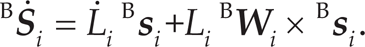
The kinematic model of the Stewart platform is shown in Fig. 1. Rotation centres of spherical joints are marked by points P₁, P₂, P₃, P₄, P₅, P₆, while rotation centres of universal joints are symbolized by B₁, B₂, B₃, B₄, B₅, B₆. The base frame { B }: O − XYZ and the end-effector frame { P }: o − xyz are located as shown in the figure. The base frame is the global coordinate system, according to which the subsequent kinematics and dynamics are established. The position of the end effector is expressed by the origin of the end-effector frame as t = [x, y, z]^T in the base frame. The posture of the end effector is described by the Roll-Pitch-Yaw angles of the Euler representation, namely, angle ψ about the X-axis, angle θ around the Y-axis and angle φ around the Z-axis, which can be converted into the rotation matrix ^BR_P as

${}^{B}R_{P} = [\begin{matrix} c φ c θ & c φ s θ s ψ - s φ c ψ & c φ s θ c ψ + s φ s ψ \\ s φ c θ & s φ s θ s ψ + c φ c ψ & s φ s θ c ψ - c φ s ψ \\ - s θ & c θ s ψ & c θ c ψ \end{matrix}]$ (1)

where s is the sine operation and c is the cosine operation.

Figure 1.

Kinematic model of the Stewart parallel manipulator

Figure 2.

Kinematic model of the ith limb

Limb local frames denoted as { U _i} and { L _i} are established in the ith limb, as shown in Fig. 2. Limb local frames are established to facilitate the definition of limb dynamic parameters, i.e., centroid and inertia. Frame { U _i} is attached to point B_i, with the x_i-axis along the limb. The unit cross product of the x_i-axis vector and the location vector b _i is defined as the y_i-axis vector. Then, the z_i-axis vector can be easily obtained by the cross product of the x_i-axis vector and the y_i-axis vector. Frame { L _i} is attached to point P_i, parallel to the local frame. Notations used in this paper will be described at the instance of first appearance. Generally, vectors and matrices are described in bold italic, while limb numbers are denoted by the subscript i. Left superscripts of symbols show coordinate systems, according to which physical quantities are described.

Next, the required kinematic parameters for the inverse dynamics are deduced. Position vector p _i of the rotation centre of spherical joint can be described in the base frame as

${}^{B}p_{i} = {}^{B}R_{P} p_{i} + t .$ (2)

Then, the limb vector ^B S _i can be derived from the difference of position vectors ^B p _i and b _i as

${}^{B}S_{i} = {}^{B}R_{P} p_{i} + t - b_{i} .$ (3)

The velocity mapping function can be found in the base frame by taking the derivative of Eq. (3) with respect to time and can be expressed as

${}^{B}{\dot{S}}_{i} = ω \times {}^{B}R_{P} p_{i} + \dot{t} .$ (4)

Additionally, ${}^{B}{\dot{S}}_{i}$ can be described in terms of the sliding velocity ${\dot{L}}_{i}$ and the angular velocity W _i under the base frame as

${}^{B}{\dot{S}}_{i} = {\dot{L}}_{i} {}^{B}s_{i} + L_{i} {}^{B}W_{i} \times {}^{B}s_{i} .$ (5)

where ^B s _i = ^B S _i / ∥^B S _i∥ is the unit limb vector, and L_i = ∥^B S _i∥ is the limb length. Taking dot and cross products of the above equation with ^Bs_i separately gives the sliding velocity and the angular velocity of the ith limb as

${\dot{L}}_{i} = {}^{B}s_{i} \cdot {}^{B}{\dot{S}}_{i},$ (6)

$W_{i} = {}^{B}s_{i} \times {}^{B}{\dot{S}}_{i} / L_{i} .$ (7)

Similarly, taking the derivative of Eqs. (6) and (7) with respect to time and the angular and sliding accelerations of the limb can be deduced as

$A_{i} = ({}^{B}s_{i} \times {}^{B}{\ddot{S}}_{i} - 2 {\dot{L}}_{i} W_{i}) / L_{i},$ (8)

${\ddot{L}}_{i} = {}^{B}{\dot{s}}_{i} \cdot {}^{B}{\dot{S}}_{i} + {}^{B}s_{i} \cdot {}^{B}{\ddot{S}}_{i} = L_{i} W_{i} \cdot W_{i} + {}^{B}s_{i} \cdot {}^{B}{\ddot{S}}_{i} .$ (9)

Linear accelerations of mass centres of upper and lower parts in the ith limb can be written in as

$a_{U i} = A_{i} \times r_{U i} + W_{i} \times (W_{i} \times r_{U i}),$ (10)

$a_{L i} = A_{i} \times r_{L}_{i} + W_{i} \times (W_{i} \times r_{L}_{i}) + \ddot{L} {}^{B}s_{i} + 2 {\dot{L}}_{i} W_{i} \times {}^{B}s_{i} .$ (11)

where $r_{U}_{i} = {}^{B}R_{U i} r_{Uo}$ , $r_{L i} = {}^{B}S_{i} + {}^{B}R_{U i} r_{Lo}$ and r _Uo, r _Lo denote centroid vectors of upper and lower parts under { U _i} and { L _i}, respectively. ^B R _Ui is the limb rotation matrix and can be obtained as ${}^{B}R_{U i} = [\begin{matrix} x_{i} & y_{i} & z_{i} \end{matrix}]$ , $x_{i} = {}^{B}s_{i}$ , $y_{i} = ({}^{B}s_{i} \times b_{i}) / ‖ {}^{B}s_{i} \times b_{i} ‖$ , $z_{i} = x_{i} \times y_{i}$

The linear acceleration of the mass centre of the end effector can be deduced in { B } as

$a_{P} = ω \times (ω \times e) + ε \times e .$ (12)

where e =^B R _P e ₀, and e ₀ is the position vector of the mass center of the end effector in { P }.

3. Dynamics

The moment of inertia I _Uo of the upper part limb is defined in { U _i} relative to its mass centre and can be described in the base frame as

$I_{U}_{i} = {}^{B}R_{U i} I_{Uo} {}^{B}R {_{U}}_{i}^{T} .$ (13)

Similarly, I _Lo denotes the moment of inertia of the lower part limb in { L _i} relative to its mass centre and can be written in the base frame as

$I_{L}_{i} = {}^{B}R_{U i} I_{Lo} {}^{B}R {_{U}}_{i}^{T} .$ (14)

The moment of inertia I _Po of the end effector in { P } relative to the mass centre can be written in the base frame as

$I_{P} = {}^{B}R_{P} I_{Po} {}^{B}R {_{P}}^{T} .$ (15)

In the base frame, relative to the base point B_i, the Euler's equation for the ith limb is derived as

$\begin{array}{l} {}^{B}S_{i} \times F_{S i} + M_{U i} {}^{B}s_{i} + (m_{L} r_{L} + m_{U} r_{U}) \times g = m_{L} r_{L} \times a_{L i} \\ + m_{U} r_{U} \times a_{U i} + (I_{L} + I_{U}) A_{i} + W_{i} \times (I_{L} + I_{U}) W_{i} . \end{array}$ (16)

where M_Ui is the mode of the constraint moment exerted by the universal joint avoiding self-rotation along the limb axis, and F _si is the constraint force of the spherical joint acting on the limb.

The above equation can be simplified as

${}^{B}S_{i} \times F_{S i} + M_{U} {}^{B}s_{i} = D_{i},$ (17)

where $\begin{array}{l} D_{i} = m_{L} r_{L} \times a_{L i} + m_{U} r_{U} \times a_{U i} + (I_{L} + I_{U}) A_{i} . \\ + W_{i} \times (I_{L} + I_{U}) W_{i} - (m_{L} r_{L} + m_{U} r_{U}) \times g \end{array}$

Taking cross products of both sides of Eq. (17) with unit vector ^B s _i leads to

$F_{S i} = C_{i} + F_{Leg}_{i} {}^{B}s_{i},$ (18)

where $C_{i} = (D_{i} \times {}^{B}s_{i}) / L_{i}$ , and $F_{Leg}_{i} = {}^{B}s_{i} \cdot F_{S}_{i}$ .

The Newton's equation for the end effector can be written as ( F _E is the external force described in the base frame)

$m_{P} g - \sum_{i = 1}^{6} F_{S}_{i} + F_{E} = m_{P} a_{P} .$ (19)

Substituting F _{S_i} with Eq. (18) results in

$\sum_{i = 1}^{6} F_{Leg i} {}^{B}s_{i} = F_{E} + m_{P} g - \sum_{i = 1}^{6} C_{i} - m_{P} a_{P} .$ (20)

Relative to the geometric centre O, Euler's equation for the end effector can be written as ( M _E is the external torque described in the base frame)

$\begin{array}{l} m_{P} e \times g + M_{E} - \sum_{i = 1}^{6} {}^{B}R_{P} p_{i} \times F_{S}_{i} \\ = m_{P} e \times a_{P} + ε I_{P} + ω \times (I_{P} ω) . \end{array}$ (21)

Substituting F _Si with Eq. (18) gives

$\begin{array}{l} M_{E} + m_{P} e \times (g - a_{P}) - I_{P} ε - ω \times (I_{P} ω) - \sum_{i = 1}^{6} {}^{B}R_{P} p_{i} \times C_{i} \\ = \sum_{i = 1}^{6} F_{Leg}_{i} {}^{B}R_{P} p_{i} \times {}^{B}s_{i} . \end{array}$ (22)

Considering Eqs. (21) and (22) together, we can obtain the inverse dynamic model of the Stewart platform. In this experiment, the pull pressure sensor is installed in the lower part of each limb, as shown in Fig. 3(b). We need to deduce the algebraic expression of the sensor force. The Newton's equation of the force sensor and components below can be given as

$F_{S i} + m_{Sen} g - F_{Sen i} = m_{Sen} a_{Sen i},$ (23)

where m_Sen is the mass of the force sensor and components below and a _Seni is the centroid acceleration of these parts, and can be obtained similarly to a _Li.

Since the pull pressure sensor can only record contribution along the limb, taking the dot product with the unit limb vector ^B s _i gives the sensor force as

$F_{i} = F_{Leg i} + Q_{i},$ (24)

where $F_{i} = {}^{B}s_{i} \cdot F_{Sen i}$ and $Q_{i} = m_{Sen} {}^{B}s_{i} \cdot (g - a_{Sen i})$

4. Dynamics Verification Experiment

The dynamics verification experiment is carried out as follows: firstly, the force sensor (pull pressure sensor) is equipped in each limb of the object Stewart platform. Next, control the end effector of the Stewart platform moving along the given trajectory and simultaneously record data from the force sensors and limb lengths. Finally, theoretical values of the limb force are calculated based on the inverse dynamics and recorded limb lengths, while practical values of the limb force are measured with force sensors using an ADC (analogue-to-digital converter). Dynamic parameters of the Stewart manipulator, such as mass, inertia matrix and centroid coordinates are obtained using the CAD identification method, and adjusted using a disassembly measure. The coincidence between theoretical and practical forces indicates the correctness of the dynamic model and parameters. Although the theory trajectory of the end effector is easier to achieve, recorded practical limb lengths are instead adopted in the experiment, which reflect the actual impacts of the interpolation algorithm, as well as the dynamic performance of the drive module. In other words, the recorded limb lengths comply with the real situation and should be used to calculate the limb forces.

The experimental platform is a typical Stewart platform, as shown in Fig. 3(a). Each limb is driven by an AC servo motor and the force sensor is equipped in each limb close to the spherical joint to measure the actual limb force, as shown in Fig. 3(b). The open CNC system is adopted to control the Stewart platform, which is mainly composed of hardware in the form of an industrial computer and a motion control card. In this experiment, the Turbo PMAC card is used, a powerful programmable multi-axis controller produced by the Delta Tau Company. The hardware structure of the control system is illustrated in Fig. 4. The closed-loop position control of the Stewart platform is carried out in the joint space. The servo motor is controlled directly by the servo driver at the velocity control mode. The servo driver is connected to the PMAC card through the JMACH1 and JMACH2, which communicates signals and instructions. The position loop of each limb is closed in the PMAC card. The PMAC card is plugged into the PCI slot of the industrial computer, which facilitates the data exchange and interrupts requests. The ACC-36P accessory is added to transfer the analogue voltage output of the force sensor to the digital signal.

Figure 3.

Physical experimental platform

The adopted CNC software of the parallel manipulator is developed based on the RTLinux (Real-Time Linux) [21] and Linux systems. The interactive interface is implemented using the MniGUI software [22]. The CNC software realizes inverse kinematics in addition to trajectory planning and coarse interpolation. The fine interpolation is carried out in the joint space by the PMAC card.

The data acquisition and delivery process is the key to the dynamics verification experiment. Length and force data of limbs should be synchronously recorded. As shown in Fig. 5, cooperation of interruption and dual-port RAM (random access memory) realizes the real-time transmission of large data. Dual-port RAM can be accessed by the CNC software and PMAC program at the same time. Data regarding limb length and force is collected automatically by the PMAC card and saved in special registers. The PLC program, which works with the PMAC card, is used to deliver the data to the dual-port ram, while the real-time thread of the RTLinux reads the data in each interruption at the period of 0.22ms. In the CNC software, circular queues are created to bridge the real-time and non-real-time sections, delivering the data to the non-real-time thread of the Linux system. Finally, data are saved by calling up the file manipulation functions of the Linux system.

Figure 4.

Hardware structure of the control system

Figure 5.

Diagram of data acquisition and delivery

In order to receive the required dynamic parameters, a practical identification method is used in this paper, which takes full advantage of the CAD model and disassembly measurements. Specifically, firstly, a detailed CAD model needs to be built; this was already completed in the design stage using UG software, as shown in Fig. 6. Then, the Stewart manipulator is disassembled, the mass of each component is weighed and the mass property of the corresponding component in the CAD model accordingly. Since limbs are identical, it is only necessary to disassemble one limb. Finally, parameters for the inertia matrix and centroid coordinate relative to the given frames can be conveniently obtained by the body measurement function of the UG software. Some parameters (e.g., friction), which change over time and due to a variety of other factors are omitted here. This is because such parameters are minor and have little impact on the dynamic calculation, which is usually compensated for in dynamic control with the adaptive algorithm [23].

In order to discuss the singularity of the Stewart manipulator, the Jacobian matrix is deduced. Considering Eqs. (4) and (5) together, we can deduce the following equation

$\dot{t} + ω \times (R p_{i}) = L_{i} W_{i} \times s_{i} + {\dot{L}}_{i} s_{i} .$ (25)

Take the dot product of Eq. (25) with the unit limb vector s _i at both sides and the velocity mapping equation can be established as

$s_{i} \cdot \dot{t} + [(R p_{i}) \times s_{i}] \cdot ω = {\dot{L}}_{i} .$ (26)

The above equation can be organized in the matrix form as

$J \dot{X} = \dot{L},$ (27)

where J is the Jacobian matrix of the Stewart parallel manipulator.

Figure 6.

Detailed CAD model of the Stewart manipulator

As shown in Eq. (27), for the Stewart platform, there is only the second type kinematic singularity, when det( J )=0. Such singularities can be further classified into three categories are adjusted, namely, architecture singularity, configuration singularity and formulation singularity [24, 25]. If the base and the end effector of the Stewart manipulator are similar polygons, an architecture singularity occurs, which should be completely avoided in the design. When the base and the end effector coincide, or if limbs are of the same length with an end-effector rotation of ±π / 2 around the Z-axis, the configuration singularity appears. The formulation singularity is generally introduced by the adopted description method of the end effector posture. In this paper, since the Euler representation is used, this type of singularity exists when the rotation angle around the Y-axis is ±π/2.

The architecture singularity can be avoided by the rational definition of the base and end-effector frames. As shown in Fig. 1(b), the base and end-effector frames are established with a difference angle of π / 3 relative to the joint distribution. Additionally, only when α = β = π / 3 can the architecture singularity appear. At the same time, the rotation angle of ±π / 2 is too large to be available for the Stewart manipulator. Thus, only the configuration singularity, where the base and the end effector coincide, must be avoided.

The workspace of our object Stewart platform is a sphere with a radius of 0.1m and the coordinates of the workspace centre is (0, 0, −0.967) m in the base frame. Thus, the kinematic singularity of the object's Stewart platform is totally avoided in the defined workspace. The experiment trajectories are within the maximum horizontal cross-section of the workspace, where the Z-axis coordinate is −0.967m. The end effector is controlled following the linear reciprocating motion along the X-axis and Y-axis, respectively, with no rotation between −50mm to 50mm. The feed speed of the end effector is 1800mm/min and the given acceleration is 1m/s².

Figure 7.

Flow chart of experimental data processing

The experimental data processing includes two aspects, as shown in Fig. 7. On the one hand, theoretical forces are calculated using the recorded limb lengths. In order to get the practical pose of the end effector, the forward kinematics [26] of the Stewart manipulator is carried out. Computing the end-effector pose is equivalent to solving equations deduced from Eq. (3), which can be written as the function of X = [x, y, z, ψ, θ, φ]^T:

$f_{i} (X) = ‖ {}^{B}R_{P} p_{i} + t - b_{i} ‖ - L_{i} = 0, i = 1, 2, \dots, 6,$ (28)

and the equation can be rewritten as

$\begin{array}{l} f_{i} (X) = p_{i}^{T} p_{i} + t^{T} t + b_{i}^{T} b_{i} + 2 t^{T} ({}^{B}R_{P} p_{i}) \\ - 2 b_{i}^{T} ({}^{B}R_{P} p_{i}) - 2 b_{i}^{T} t - L_{i}^{2} . \end{array}$

Since the above equations present difficulties for achieving the algebra root, the Newton-Raphson method [27] is adopted for receiving numerical solutions. The above equation can be expressed in matrix form as

$F (X) = {[f_{1}, f_{2}, f_{3}, f_{4}, f_{5}, f_{6}]}^{T} = 0.$ (29)

In order to facilitate calculation, let us define a matrix K as

$K = [\begin{matrix} \frac{\partial f_{1}}{\partial X (1)} & \dots & \frac{\partial f_{1}}{\partial X (6)} \\ ⋮ & ⋱ & ⋮ \\ \frac{\partial f_{6}}{\partial X (1)} & \dots & \frac{\partial f_{6}}{\partial X (6)} \end{matrix}] .$ (30)

The solution to matrix K is trivial and is in fact realized automatically using the diff function in the Matlab software.

Following on, the iterative process can be summarized as shown in Fig. 8. In order to speed up convergence, the final pose of the end effect is adopted as the initial value of the iterative routine in order to deduce the current pose.

Figure 8.

Flowchart of the iterative routine

Then, the velocity and acceleration of the end effector can be obtained by difference calculations of the pose. Finally, adopting the deduced dynamic model, theoretical values of the limb force can be realized.

On the other hand, force sensor data are refined to receive the measured value. The input range of the pull pressure sensor is 0∼±500N and its output is the bipolar analogue voltage signal of 0∼±5V. An ADC with a resolution of 12 bits is used in conjunction with each force sensor. Thus, the force resolution of the experiment system is 0.244N (500/2047 N). In order to eliminate the effects of the preload on each force sensor, the initial static bias of each sensor is subtracted in the adjusted static bias step. Finally, the experiment data are down-sampled by a factor of 5 and smoothed by the five-point moving average method to suppress noise introduced by both the high-frequency signal acquisition and difference calculations [28].

5. Results and Discussion

In order to facilitate a comparison, the measured (or practical) and calculated (or theoretical) values of each limb force are illustrated in Figs. 9 and 10. Corresponding trajectories of the end effector are shown along the X-axis and Y-axis, respectively. The red bold curves indicate theoretical values calculated through the inverse dynamics, while the blue slim curves indicate measured values acquired from pull pressure sensors.

The end-effector trajectory of Fig. 9 can be subdivided into three segments. In the first segment, the end effector moves along the negative direction of the Z-axis of the base frame from the machine origin to the workspace centre (the starting point of the desired reciprocating trajectory) at the fast-feed speed. Since the structure of the Stewart manipulator is circularly symmetric, the force curve of each limb is the same in this segment. The second segment starts at 4.3s and lasts until 11.0s. The end effector moves along the X-axis from the workspace centre through points (50, 0, −967) mm and (−50, 0, −967) mm in order, and stops at workspace centre. In the third section, the end effector remains motionless at the workspace centre following the above motion.

The end-effector trajectory corresponding to Fig. 10 can also be subdivided into three segments. The first and third segments are the same, and exhibit the trajectory explained above. In the second segment, the end effector moves from the workspace centre along the Y-axis, back and forth twice between points (0, 50, −967) mm and (0, −50, −967) mm, and finally stops at the workspace centre. The second segment starts from 4.3s and continues to 17.6s. As shown in Fig. 1, the limbs of the Stewart manipulator distribute symmetrically, relative to the Y-axis. Thus, the forces of limbs 6, 1 and 2 are the same as the forces of limb 5, 4 and 3, respectively.

As shown in Figs. 9 and 10, both calculated and measured force curves contain ripples when the end effector completes uniform linear motion, and this phenomenon is more obvious in the measured force curves. However, if limb forces are calculated according to the inputted theory trajectory, the force curves must be smooth. This phenomenon is mainly due to the adopted control method and dynamics of the drive system.

On the one hand, the coarse interpolation of the Stewart manipulator is carried out in the operating space. Then, following the inverse kinematics, fine interpolation is implemented in the joint space. Error-based tracking control and nonlinear kinematics causes the limb velocity to change even when the end effector follows the uniform linear motion. The limb velocity is adjusted minutely and frequently to meet the required terminal trajectory accuracy. Thus, the limb force changes accordingly.

Figure 9.

Experiment results when the end effector moves along the X-axis

Figure 10.

Experiment results when the end effector moves along the Y-axis

On the other hand, the classic closed-loop position control system is adopted, which consists of a position loop, speed loop and current loop (or force loop). The current loop is closed internally and possesses the fastest response frequency. In other words, the force of each limb changes

Table 1.

Differences between the calculated force and measured force of each limb

		Force of limb 1 (N)	Force of limb 2 (N)	Force of limb 3 (N)	Force of limb 4 (N)	Force of limb 5 (N)	Force of limb 6 (N)
End effector moves along X-axis	RMS difference	0.696	1.148	1.242	0.793	1.007	0.8016
End effector moves along X-axis	Max difference	3.268	5.650	6.150	2.968	6.220	4.216
End effector moves along Y-axis	RMS difference	1.377	0.746	0.926	1.516	1.097	1.043
End effector moves along Y-axis	Max difference	5.364	2.753	6.591	6.310	4.671	4.960

more intensively and rapidly than the length does. Thus, compared with the calculated force curve that is deduced from the limb length, the measured force curve fluctuates more significantly, with more saw teeth and spikes. In other words, it is quite natural for there to be small transient differences between the calculated force curve and the measured force curve.

Differences between calculated forces and measured forces are summarized in Table 1, and are quite small. The maximum RMS (root mean square) difference between measured and calculated forces is 1.516N, which appears in the force curve of the fourth limb when the end effector moves along the Y-axis. The maximum difference is 6.591N, which happens in the force curve of the third limb when the end effector moves along the X-axis. Generally, the curve of measured force coincides well with the curve of calculated force, especially during acceleration and deceleration phases. Thus, it is reasonable to conclude that the deduced inverse dynamics and parameters of the Stewart manipulator are correct.

6. Conclusions

In this paper, a dynamics verification experiment is carried out on the Stewart platform. Firstly, the complete dynamic model of the Stewart manipulator is established using the classic Newton-Euler method and considering the force sensors. Then, inertia and centroid properties of the Stewart platform are obtained using the practical identification approach, without depending on expensive instruments or complex calculations. Finally, with the developed physical experiment platform, dynamic model and obtained parameters are verified by comparing theoretically calculated limb forces with actual measured limb forces.

Experiment results are analysed and reveal that due to the position interpolation algorithm and dynamics of the drive system, the actual trajectory of the Stewart platform is different from the theory trajectory inputted into the CNC system, and the limb force curve naturally contain ripples. Since each limb of the Stewart platform is controlled by the traditional closed-loop position system and the force loop is the inner of these, it is reasonable to conclude that the measured force curves fluctuate more significantly than the force curves calculated from the practical limb length. In the follow-up study, the torque control mode of servo motors will be applied to the Stewart platform in order to build up the adaptive controller for researching the dynamic control of the Stewart platform.

The dynamics verification algorithm proposed and illustrated in this paper, which involves dynamic modelling, a data analysis method and parameter identification approach is generic and practical, and can be flexibly applied to the dynamic analysis of other parallel manipulators.

Footnotes

7.

This research is sponsored by the National Natural Science Foundation of China (No. 51205224,51475252,51575292) and Tsinghua University Initiative Scientific Research Program (No.2014z22068).

References

Tsai

L W.

Robot Analysis, The Mechanics of Serial and Parallel Manipulators. New York: Wiley, pp. 19–28, 1999.

Wohlhart

Mobile 6-SPS parallel manipulators. Journal of Robotic Systems, 20(8), pp. 509–516, 2003.

Merlet

J P.

Parallel Robots (2nd Ed.). Netherlands: Springer, pp. 69–92, 2006.

Tang

Wang

and Gao

Kinematic calibration of gantry hybrid machine tool based on estimation error and local measurement information. International Journal of Advanced Manufacturing Technology, 26(4), pp. 382–390, 2005.

Weck

Staimer

Parallel kinematic machine tools – current state and future potentials. CIRP Annals – Manufacturing Technology, 51(2), pp. 671–683, 2002.

Shao

Z-F

Tang

Wang

L-P

Chen

Dynamic modeling and wind vibration control of the feed support system in FAST. Nonlinear Dynamics, 67(2), pp. 965–985, 2011.

Taghirad

H D

Nahon

Dynamic analysis of a macro-micro redundantly actuated parallel manipulator. Advanced Robotics, 24, pp. 949–981, 2008.

D S

and Gu

H B.

Adaptive sliding control of six-DOF flight simulator motion platform. Chinese Journal of Aeronaurics, 20(5), pp. 425–433, 2007.

Bonev

I A.

The true origins of parallel robots. http://www.parallemic.org/Reviews/Review007.html. Accessed on 10 Sep 2015.

10.

Huang

Chetwynd

D G

Gosselin

C M.

Conceptual design and dimensional synthesis of a novel 2-DOF translational parallel robot for pick-and-place operations. Journal of Mechanical Design, 126(3), pp. 449–455, 2004.

11.

Pierrot

Reynaud

Fournier

DELTA: a simple and efficient parallel robot. Robotica, 8(2), pp. 105–109, 2009.

12.

Wang

L-P

Wang

Dynamic formulation of a planar 3-DOF parallel manipulator with actuation redundancy. Robotics and Computer-Integrated Manufacturing, 26(1), pp. 67–73, 2010.

13.

Hong

Yamamoto

A calculation method of the reaction force and moment for a Delta-type parallel link robot fixed with a frame. Robotica, 27(4), pp. 579–587, 2009.

14.

Staicu

Dynamic of the 6-6 Stewart parallel manipulator. Robotics and Computer-Integrated Manufacturing, 27(1), pp. 212–220, 2011.

15.

Wang

Gosselin

C M.

A new approach for the dynamic analysis of parallel manipulators. Multibody System Dynamics, 2(3), pp. 317–334, 1998.

16.

Staicu

Liu

X-J

Explicit dynamics equations of the constrained robotic systems. Nonlinear Dynamics, 58(1–2), pp. 217–235, 2009.

17.

Shao

Tang

Chen

Wang

Inertia match research of a 3-RRR reconfigurable planar parallel manipulator. Chinese Journal of Mechanical Engineering, 28(6), pp. 649–659, 2012.

18.

Yuan

Multi-degree of freedom vibration model for a 3-DOF hybrid robot. In: Proceedings of 2009 IEEE/ASME International Conference on Advanced Intelligent Mechatronics. Singapore: Singapore, pp. 1474–1479, 2009.

19.

Dasgupta

Mruthyunjaya

T S.

The Stewart platform manipulator: a review. Mechanism and Machine Theory, 35(1), pp. 15–40, 2000.

20.

Stewart

A platform with six degrees of freedom. In: Proceedings of the Institution of Mechanical Engineers. Britain: London, 1(15), pp. 371–386, 1965.

21.

Petrosino

Miralto

Ferone

A real-time streaming server in the RTLinux environment using VideoLanClient. Journal of Real-Time Image Processing, 6(4), pp. 247–256, 2011.

22.

http://www.minigui.org/en/. Accessed on 10 Sep 2015.

23.

Cazalilla

Valles

Mata

Diaz-Rodriguez

Valera

Adaptive control of a 3-DOF parallel manipulator considering payload handling and relevant parameter models. Robotics and Computer-Integrated Manufacturing, 30(5), pp. 468–477, 2014.

24.

Gosselin

Angeles

Singularity analysis of closed-loop kinematic chains. IEEE Transaction on Robotics and Automation, 6(3), pp. 281–290, 1990.

25.

Wen

J T

O'Brien

J F.

Singularities in Three-legged Platform-type Parallel Mechanisms. IEEE Transactions on Robotics and Automation, 19(4), pp. 720–727, 2003.

26.

Freitas

G M

Leite

A C

Lizarralde

Kinematic Control of Constrained Robotic Systems. Control and Automation Magazine of the Brazilian Automatic Society, 22(6), pp. 559–572, 2011.

27.

Yang

C-F.

Forward kinematics analysis of parallel manipulator using modified global Newton-Raphson method. Journal of Central South University of Technology (English Edition), 17(6), pp. 1264–1270, 2010.

28.

Zhang

Fan

and Wang

Vibration analysis of rolling mill based on signal-frequency characteristics. Journal of Vibration, Measurement & Diagnosis, 3(5), pp. 642–646, 2011.